
Allen-Cahn equation#
Problem setup#
We will solve an Allen-Cahn equation:
The initial condition is defined as the following: $\( u(x, 0) = x^2\cos(\pi x) \)$
And the boundary condition is defined: $\( u(-1, t) = u(1, t) = -1 \)$
The reference solution is here.
Because the Allen-Cahn equation has inconsistent units, so here we do not provide the physical meaning of the parameters.
Implementation#
This description goes through the implementation of a solver for the above described Allen-Cahn equation step-by-step.
First, Import the necessary library used for this project:
import brainstate
import braintools
import brainunit as u
import numpy as np
from scipy.io import loadmat

import pinnx
We then begin by defining a computational geometry and a time domain. We can use a built-in class Interval and TimeDomain, and we can combine both of the domains using GeometryXTime.
geom = pinnx.geometry.Interval(-1, 1)
timedomain = pinnx.geometry.TimeDomain(0, 1)
geomtime = pinnx.geometry.GeometryXTime(geom, timedomain).to_dict_point('x', 't')
Now, we express the PDE residual of the Allen-Cahn equation:
d = 0.001

@brainstate.transform.jit
def pde(x, out):
    jacobian = net.jacobian(x)
    hessian = net.hessian(x, xi='x', xj='x')
    dy_t = jacobian['u']['t']
    dy_xx = hessian['u']['x']['x']
    return dy_t - d * dy_xx - 5 * (out['u'] - out['u'] ** 3)
Next, we choose the network. Here, we use a fully connected neural network of depth 4 (i.e., 3 hidden layers) and width 20:
net = pinnx.nn.Model(
    pinnx.nn.DictToArray(x=None, t=None),
    pinnx.nn.FNN(
        [2] + [20] * 3 + [1],
        activation="tanh",
        output_transform=lambda x, y: u.math.expand_dims(
            x[..., 0] ** 2 * u.math.cos(np.pi * x[..., 0]) +
            x[..., 1] * (1 - x[..., 0] ** 2) * y,
            axis=-1
        )
    ),
    pinnx.nn.ArrayToDict(u=None)
)
The first argument to pde is a 2-dimensional vector where the first component(x[:, 0]) is x-coordinate and the second component (x[:, 1]) is the t-coordinate. The second argument is the network output, i.e., the solution u(x, t), but here we use y as the name of the variable.
Now that we have specified the geometry and PDE residual, we can define the TimePDE problem as the following:
problem = pinnx.problem.TimePDE(
    geomtime,
    pde,
    [],
    net,
    num_domain=8000,
    num_boundary=400,
    num_initial=800
)
Now that we have defined the neural network, we build a Model, choose the optimizer and learning rate (lr), and train it for 15000 iterations:
trainer = pinnx.Trainer(problem)
trainer.compile(braintools.optim.Adam(lr=1e-3)).train(iterations=15000)
Compiling trainer...
'compile' took 0.057796 s

Training trainer...

Step      Train loss                                 Test loss                                  Test metric
0         [Array(1.2709892, dtype=float32)]          [Array(1.2709892, dtype=float32)]          []
1000      [Array(0.5983757, dtype=float32)]          [Array(0.5983757, dtype=float32)]          []
2000      [Array(0.5952873, dtype=float32)]          [Array(0.5952873, dtype=float32)]          []
3000      [Array(0.5927927, dtype=float32)]          [Array(0.5927927, dtype=float32)]          []
4000      [Array(0.58992064, dtype=float32)]         [Array(0.58992064, dtype=float32)]         []
5000      [Array(0.58779794, dtype=float32)]         [Array(0.58779794, dtype=float32)]         []
6000      [Array(0.5867402, dtype=float32)]          [Array(0.5867402, dtype=float32)]          []
7000      [Array(0.5860185, dtype=float32)]          [Array(0.5860185, dtype=float32)]          []
8000      [Array(0.58559114, dtype=float32)]         [Array(0.58559114, dtype=float32)]         []
9000      [Array(0.5853089, dtype=float32)]          [Array(0.5853089, dtype=float32)]          []
10000     [Array(0.58509886, dtype=float32)]         [Array(0.58509886, dtype=float32)]         []
11000     [Array(0.5849413, dtype=float32)]          [Array(0.5849413, dtype=float32)]          []
12000     [Array(0.5848149, dtype=float32)]          [Array(0.5848149, dtype=float32)]          []
13000     [Array(0.5847117, dtype=float32)]          [Array(0.5847117, dtype=float32)]          []
14000     [Array(0.5846201, dtype=float32)]          [Array(0.5846201, dtype=float32)]          []
15000     [Array(0.5845136, dtype=float32)]          [Array(0.5845136, dtype=float32)]          []

Best trainer at step 15000:
  train loss: 5.85e-01
  test loss: 5.85e-01
  test metric: []

'train' took 2405.874751 s
<pinnx.Trainer at 0x12c317e50>
After we train the network using Adam, we continue to train the network using L-BFGS to achieve a smaller loss:
trainer.compile(braintools.optim.LBFGS(lr=1e-3)).train(1000, display_every=200)
Compiling trainer...
'compile' took 0.198848 s

Training trainer...

Step      Train loss                                 Test loss                                  Test metric
15000     [Array(0.5845136, dtype=float32)]          [Array(0.5845136, dtype=float32)]          []
15200     [Array(0.5845137, dtype=float32)]          [Array(0.5845137, dtype=float32)]          []
15400     [Array(0.5845137, dtype=float32)]          [Array(0.5845137, dtype=float32)]          []
15600     [Array(0.5845136, dtype=float32)]          [Array(0.5845136, dtype=float32)]          []
15800     [Array(0.58451355, dtype=float32)]         [Array(0.58451355, dtype=float32)]         []
16000     [Array(0.58451355, dtype=float32)]         [Array(0.58451355, dtype=float32)]         []

Best trainer at step 15800:
  train loss: 5.85e-01
  test loss: 5.85e-01
  test metric: []

'train' took 150.270458 s
<pinnx.Trainer at 0x12c317e50>
We then save and plot the best trained result and the loss history of the model.
trainer.saveplot(issave=True, isplot=True)
Saving loss history to /Users/sichaohe/Documents/GitHub/pinnx/docs/examples-pinn-forward/loss.dat ...
Saving checkpoint into /Users/sichaohe/Documents/GitHub/pinnx/docs/examples-pinn-forward/loss.dat
Saving training data to /Users/sichaohe/Documents/GitHub/pinnx/docs/examples-pinn-forward/train.dat ...
Saving checkpoint into /Users/sichaohe/Documents/GitHub/pinnx/docs/examples-pinn-forward/train.dat
Saving test data to /Users/sichaohe/Documents/GitHub/pinnx/docs/examples-pinn-forward/test.dat ...
Saving checkpoint into /Users/sichaohe/Documents/GitHub/pinnx/docs/examples-pinn-forward/test.dat
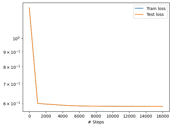
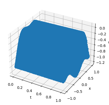
Next, we load and prepare the dataset with gen_testdata(). Finally, we test the model and display a graph containing both training loss and testing loss over time. We also display a graph containing the predicted solution to the PDE.
def gen_testdata():
    data = loadmat("../dataset/Allen_Cahn.mat")

    t = data["t"]
    x = data["x"]
    u = data["u"]

    xx, tt = np.meshgrid(x, t)
    X = dict(x=np.ravel(xx), t=np.ravel(tt))
    return X, u.flatten()


X, y_true = gen_testdata()
y_pred = trainer.predict(X)
f = pde(X, y_pred)

print(y_true.shape, y_pred['u'].shape)
print("Mean residual:", u.math.mean(u.math.absolute(f)))
print("L2 relative error:", braintools.metric.l2_norm(y_true, y_pred['u']))
(20301,) (20301, 20301)
Mean residual: 0.5783491
---------------------------------------------------------------------------
AssertionError                            Traceback (most recent call last)
Cell In[12], line 19
     17 print(y_true.shape, y_pred['u'].shape)
     18 print("Mean residual:", u.math.mean(u.math.absolute(f)))
---> 19 print("L2 relative error:", braintools.metric.l2_norm(y_true, y_pred['u']))

File ~/miniconda3/envs/pinnx/lib/python3.11/site-packages/braintools/metric/_regression.py:300, in l2_norm(predictions, targets, axis)
    297 assert bu.math.is_float(predictions), 'predictions must be float.'
    298 if targets is not None:
    299   # Avoid broadcasting logic for "-" operator.
--> 300   assert predictions.shape == targets.shape, 'predictions and targets must have the same shape.'
    301 errors = predictions - targets if targets is not None else predictions
    302 return jnp.linalg.norm(errors, axis=axis, ord=2)

AssertionError: predictions and targets must have the same shape.