
Burgers equation#
Problem setup#
We will solve a Burgers equation:
with the Dirichlet boundary conditions and initial conditions
Dimensional Analysis#
Step 1: Assign Dimensions to Variables#
Spatial Coordinate \(x\):
The dimension of \(x\) is length:
\[ [x] = L. \]
Time \(t\):
The dimension of time is:
\[ [t] = T. \]
Velocity \(u\):
Velocity has dimensions of length per unit time:
\[ [u] = L / T. \]
Viscosity \(\nu\):
The term \(\nu \frac{\partial^2 u}{\partial x^2}\) involves the second spatial derivative of velocity, which must have the same dimensions as the time derivative \(\frac{\partial u}{\partial t}\).
Step 2: Analyze the Dimensions of Each Term#
Time Derivative Term:
The time derivative \(\frac{\partial u}{\partial t}\) has dimensions:
\[ \left[\frac{\partial u}{\partial t}\right] = \frac{[u]}{[t]} = \frac{L / T}{T} = \frac{L}{T^2}. \]
Advection Term:
The advection term \(u \frac{\partial u}{\partial x}\) involves the spatial derivative of velocity:
\[ \left[u \frac{\partial u}{\partial x}\right] = [u] \cdot \frac{[u]}{[x]} = \frac{L}{T} \cdot \frac{L / T}{L} = \frac{L}{T^2}. \]
Diffusion Term:
The diffusion term \(\nu \frac{\partial^2 u}{\partial x^2}\) involves the second spatial derivative of velocity:
\[ \left[\frac{\partial^2 u}{\partial x^2}\right] = \frac{[u]}{[x]^2} = \frac{L / T}{L^2} = \frac{1}{L T}. \]Therefore, the diffusion term has dimensions:
\[ \left[\nu \frac{\partial^2 u}{\partial x^2}\right] = [\nu] \cdot \frac{1}{L T} = \frac{L}{T^2}. \]
Step 3: Determine the Dimensions of \(\nu\)#
The diffusion term \(\nu \frac{\partial^2 u}{\partial x^2}\) must have the same dimensions as the time derivative \(\frac{\partial u}{\partial t}\):
\[ [\nu] \cdot \frac{1}{L T} = \frac{L}{T^2} \implies [\nu] = \frac{L^2}{T}. \]Therefore, the viscosity \(\nu\) has dimensions of kinematic viscosity:
\[ [\nu] = \frac{L^2}{T}. \]
Step 4: Summary of Dimensions#
Variable/Parameter |
Physical Meaning |
Dimensions |
|---|---|---|
\(x\) |
Spatial coordinate |
\(L\) |
\(t\) |
Time |
\(T\) |
\(u\) |
Velocity |
\(L / T\) |
\(\nu\) |
Kinematic viscosity |
\(L^2 / T\) |
Step 5: Initial and Boundary Conditions#
Boundary Conditions:
The boundary conditions \(u(-1,t) = u(1,t) = 0\) are given in meters per second:
\[ [u(-1,t)] = [u(1,t)] = L / T. \]
Initial Condition:
The initial condition \(u(x,0) = -\sin(\pi x)\) is given in meters per second:
\[ [u(x,0)] = L / T. \]The term \(\sin(\pi x)\) is dimensionless because \(x\) is in meters, and \(\pi\) is a dimensionless constant.
Implementation#
This description goes through the implementation of a solver for the above described Burgers equation step-by-step.
First, import the libraries we need:
import braintools
import brainunit as u
import numpy as np
import pinnx
We begin by defining a computational geometry and time domain. We can use a built-in class Interval and TimeDomain and we combine both the domains using GeometryXTime as follows:
geometry = pinnx.geometry.GeometryXTime(
    geometry=pinnx.geometry.Interval(-1., 1.),
    timedomain=pinnx.geometry.TimeDomain(0., 0.99)
).to_dict_point(x=u.meter, t=u.second)
Next, we express the PDE residual of the Burgers equation:
v = 0.01 / u.math.pi * u.meter ** 2 / u.second


def pde(x, y):
    jacobian = approximator.jacobian(x)
    hessian = approximator.hessian(x)
    dy_x = jacobian['y']['x']
    dy_t = jacobian['y']['t']
    dy_xx = hessian['y']['x']['x']
    residual = dy_t + y['y'] * dy_x - v * dy_xx
    return residual
Next, we consider the boundary/initial condition. on_boundary is chosen here to use the whole boundary of the computational domain in considered as the boundary condition. We include the geomtime space, time geometry created above and on_boundary as the BCs in the DirichletBC function of DeepXDE. We also define IC which is the inital condition for the burgers equation and we use the computational domain, initial function, and on_initial to specify the IC.
uy = u.meter / u.second

bc = pinnx.icbc.DirichletBC(lambda x: {'y': 0. * uy})
ic = pinnx.icbc.IC(lambda x: {'y': -u.math.sin(u.math.pi * x['x'] / u.meter) * uy})
Next, we choose the network. Here, we use a fully connected neural network of depth 4 (i.e., 3 hidden layers) and width 20:
approximator = pinnx.nn.Model(
    pinnx.nn.DictToArray(x=u.meter, t=u.second),
    pinnx.nn.FNN(
        [geometry.dim] + [20] * 3 + [1],
        "tanh",
        braintools.init.KaimingUniform()
    ),
    pinnx.nn.ArrayToDict(y=uy)
)
Now, we have specified the geometry, PDE residual, and boundary/initial condition. We then define the TimePDE problem as
problem = pinnx.problem.TimePDE(
    geometry,
    pde,
    [bc, ic],
    approximator,
    num_domain=2540,
    num_boundary=80,
    num_initial=160,
)
The number 2540 is the number of training residual points sampled inside the domain, and the number 80 is the number of training points sampled on the boundary. We also include 160 initial residual points for the initial conditions.
Now, we have the PDE problem and the network. We build a Trainer and choose the optimizer and learning rate:
trainer = pinnx.Trainer(problem)
trainer.compile(braintools.optim.Adam(1e-3)).train(iterations=15000)
Compiling trainer...
'compile' took 0.047883 s

Training trainer...

Step      Train loss                                                  Test loss                                                   Test metric
0         [0.15803409 * 10.0^0 * ((meter / second) / second) ** 2,    [0.15803409 * 10.0^0 * ((meter / second) / second) ** 2,    []
           {'ibc0': {'y': 0.25960198 * meter / second}},               {'ibc0': {'y': 0.25960198 * meter / second}},
           {'ibc1': {'y': 1.1659584 * meter / second}}]                {'ibc1': {'y': 1.1659584 * meter / second}}]
1000      [0.04754296 * 10.0^0 * ((meter / second) / second) ** 2,    [0.04754296 * 10.0^0 * ((meter / second) / second) ** 2,    []
           {'ibc0': {'y': 0.00308682 * meter / second}},               {'ibc0': {'y': 0.00308682 * meter / second}},
           {'ibc1': {'y': 0.06809452 * meter / second}}]               {'ibc1': {'y': 0.06809452 * meter / second}}]
2000      [0.04182805 * 10.0^0 * ((meter / second) / second) ** 2,    [0.04182805 * 10.0^0 * ((meter / second) / second) ** 2,    []
           {'ibc0': {'y': 0.00125541 * meter / second}},               {'ibc0': {'y': 0.00125541 * meter / second}},
           {'ibc1': {'y': 0.05376936 * meter / second}}]               {'ibc1': {'y': 0.05376936 * meter / second}}]
3000      [0.03440975 * 10.0^0 * ((meter / second) / second) ** 2,    [0.03440975 * 10.0^0 * ((meter / second) / second) ** 2,    []
           {'ibc0': {'y': 0.00054205 * meter / second}},               {'ibc0': {'y': 0.00054205 * meter / second}},
           {'ibc1': {'y': 0.04500021 * meter / second}}]               {'ibc1': {'y': 0.04500021 * meter / second}}]
4000      [0.0215442 * 10.0^0 * ((meter / second) / second) ** 2,     [0.0215442 * 10.0^0 * ((meter / second) / second) ** 2,     []
           {'ibc0': {'y': 0.00029352 * meter / second}},               {'ibc0': {'y': 0.00029352 * meter / second}},
           {'ibc1': {'y': 0.03042006 * meter / second}}]               {'ibc1': {'y': 0.03042006 * meter / second}}]
5000      [0.01140877 * 10.0^0 * ((meter / second) / second) ** 2,    [0.01140877 * 10.0^0 * ((meter / second) / second) ** 2,    []
           {'ibc0': {'y': 0.00016095 * meter / second}},               {'ibc0': {'y': 0.00016095 * meter / second}},
           {'ibc1': {'y': 0.02001206 * meter / second}}]               {'ibc1': {'y': 0.02001206 * meter / second}}]
6000      [0.00863622 * 10.0^0 * ((meter / second) / second) ** 2,    [0.00863622 * 10.0^0 * ((meter / second) / second) ** 2,    []
           {'ibc0': {'y': 9.4245006e-05 * meter / second}},            {'ibc0': {'y': 9.4245006e-05 * meter / second}},
           {'ibc1': {'y': 0.01318286 * meter / second}}]               {'ibc1': {'y': 0.01318286 * meter / second}}]
7000      [0.00690631 * 10.0^0 * ((meter / second) / second) ** 2,    [0.00690631 * 10.0^0 * ((meter / second) / second) ** 2,    []
           {'ibc0': {'y': 5.483637e-05 * meter / second}},             {'ibc0': {'y': 5.483637e-05 * meter / second}},
           {'ibc1': {'y': 0.00822749 * meter / second}}]               {'ibc1': {'y': 0.00822749 * meter / second}}]
8000      [0.00483667 * 10.0^0 * ((meter / second) / second) ** 2,    [0.00483667 * 10.0^0 * ((meter / second) / second) ** 2,    []
           {'ibc0': {'y': 2.3079416e-05 * meter / second}},            {'ibc0': {'y': 2.3079416e-05 * meter / second}},
           {'ibc1': {'y': 0.00571595 * meter / second}}]               {'ibc1': {'y': 0.00571595 * meter / second}}]
9000      [0.00386771 * 10.0^0 * ((meter / second) / second) ** 2,    [0.00386771 * 10.0^0 * ((meter / second) / second) ** 2,    []
           {'ibc0': {'y': 1.4185833e-05 * meter / second}},            {'ibc0': {'y': 1.4185833e-05 * meter / second}},
           {'ibc1': {'y': 0.00445467 * meter / second}}]               {'ibc1': {'y': 0.00445467 * meter / second}}]
10000     [0.00332004 * 10.0^0 * ((meter / second) / second) ** 2,    [0.00332004 * 10.0^0 * ((meter / second) / second) ** 2,    []
           {'ibc0': {'y': 1.3227182e-05 * meter / second}},            {'ibc0': {'y': 1.3227182e-05 * meter / second}},
           {'ibc1': {'y': 0.00389429 * meter / second}}]               {'ibc1': {'y': 0.00389429 * meter / second}}]
11000     [0.00295054 * 10.0^0 * ((meter / second) / second) ** 2,    [0.00295054 * 10.0^0 * ((meter / second) / second) ** 2,    []
           {'ibc0': {'y': 1.3391712e-05 * meter / second}},            {'ibc0': {'y': 1.3391712e-05 * meter / second}},
           {'ibc1': {'y': 0.00342724 * meter / second}}]               {'ibc1': {'y': 0.00342724 * meter / second}}]
12000     [0.00252938 * 10.0^0 * ((meter / second) / second) ** 2,    [0.00252938 * 10.0^0 * ((meter / second) / second) ** 2,    []
           {'ibc0': {'y': 1.0651251e-05 * meter / second}},            {'ibc0': {'y': 1.0651251e-05 * meter / second}},
           {'ibc1': {'y': 0.00329811 * meter / second}}]               {'ibc1': {'y': 0.00329811 * meter / second}}]
13000     [0.00229796 * 10.0^0 * ((meter / second) / second) ** 2,    [0.00229796 * 10.0^0 * ((meter / second) / second) ** 2,    []
           {'ibc0': {'y': 8.255725e-06 * meter / second}},             {'ibc0': {'y': 8.255725e-06 * meter / second}},
           {'ibc1': {'y': 0.00314907 * meter / second}}]               {'ibc1': {'y': 0.00314907 * meter / second}}]
14000     [0.00211558 * 10.0^0 * ((meter / second) / second) ** 2,    [0.00211558 * 10.0^0 * ((meter / second) / second) ** 2,    []
           {'ibc0': {'y': 6.807138e-06 * meter / second}},             {'ibc0': {'y': 6.807138e-06 * meter / second}},
           {'ibc1': {'y': 0.002992 * meter / second}}]                 {'ibc1': {'y': 0.002992 * meter / second}}]
15000     [0.002326 * 10.0^0 * ((meter / second) / second) ** 2,      [0.002326 * 10.0^0 * ((meter / second) / second) ** 2,      []
           {'ibc0': {'y': 7.791486e-06 * meter / second}},             {'ibc0': {'y': 7.791486e-06 * meter / second}},
           {'ibc1': {'y': 0.00277965 * meter / second}}]               {'ibc1': {'y': 0.00277965 * meter / second}}]

Best trainer at step 15000:
  train loss: 5.11e-03
  test loss: 5.11e-03
  test metric: []

'train' took 123.689102 s
<pinnx.Trainer at 0x24d2849f7d0>
After we train the network using Adam, we continue to train the network using L-BFGS to achieve a smaller loss:
trainer.compile(braintools.optim.LBFGS(1e-3)).train(2000, display_every=200)
Compiling trainer...
'compile' took 0.105205 s

Training trainer...

Step      Train loss                                                Test loss                                                 Test metric
15000     [0.002326 * 10.0^0 * ((meter / second) / second) ** 2,    [0.002326 * 10.0^0 * ((meter / second) / second) ** 2,    []
           {'ibc0': {'y': 7.791486e-06 * meter / second}},           {'ibc0': {'y': 7.791486e-06 * meter / second}},
           {'ibc1': {'y': 0.00277965 * meter / second}}]             {'ibc1': {'y': 0.00277965 * meter / second}}]
15200     [0.00468681 * 10.0^0 * ((meter / second) / second) ** 2,  [0.00468681 * 10.0^0 * ((meter / second) / second) ** 2,  []
           {'ibc0': {'y': 6.556747e-06 * meter / second}},           {'ibc0': {'y': 6.556747e-06 * meter / second}},
           {'ibc1': {'y': 0.00299743 * meter / second}}]             {'ibc1': {'y': 0.00299743 * meter / second}}]
15400     [0.00374917 * 10.0^0 * ((meter / second) / second) ** 2,  [0.00374917 * 10.0^0 * ((meter / second) / second) ** 2,  []
           {'ibc0': {'y': 5.420788e-06 * meter / second}},           {'ibc0': {'y': 5.420788e-06 * meter / second}},
           {'ibc1': {'y': 0.00296684 * meter / second}}]             {'ibc1': {'y': 0.00296684 * meter / second}}]
15600     [0.00311677 * 10.0^0 * ((meter / second) / second) ** 2,  [0.00311677 * 10.0^0 * ((meter / second) / second) ** 2,  []
           {'ibc0': {'y': 4.825496e-06 * meter / second}},           {'ibc0': {'y': 4.825496e-06 * meter / second}},
           {'ibc1': {'y': 0.00294279 * meter / second}}]             {'ibc1': {'y': 0.00294279 * meter / second}}]
15800     [0.00269283 * 10.0^0 * ((meter / second) / second) ** 2,  [0.00269283 * 10.0^0 * ((meter / second) / second) ** 2,  []
           {'ibc0': {'y': 4.55498e-06 * meter / second}},            {'ibc0': {'y': 4.55498e-06 * meter / second}},
           {'ibc1': {'y': 0.00292296 * meter / second}}]             {'ibc1': {'y': 0.00292296 * meter / second}}]
16000     [0.00241696 * 10.0^0 * ((meter / second) / second) ** 2,  [0.00241696 * 10.0^0 * ((meter / second) / second) ** 2,  []
           {'ibc0': {'y': 4.4667136e-06 * meter / second}},          {'ibc0': {'y': 4.4667136e-06 * meter / second}},
           {'ibc1': {'y': 0.00290674 * meter / second}}]             {'ibc1': {'y': 0.00290674 * meter / second}}]
16200     [0.00223442 * 10.0^0 * ((meter / second) / second) ** 2,  [0.00223442 * 10.0^0 * ((meter / second) / second) ** 2,  []
           {'ibc0': {'y': 4.4755107e-06 * meter / second}},          {'ibc0': {'y': 4.4755107e-06 * meter / second}},
           {'ibc1': {'y': 0.00289299 * meter / second}}]             {'ibc1': {'y': 0.00289299 * meter / second}}]
16400     [0.00212654 * 10.0^0 * ((meter / second) / second) ** 2,  [0.00212654 * 10.0^0 * ((meter / second) / second) ** 2,  []
           {'ibc0': {'y': 4.4758385e-06 * meter / second}},          {'ibc0': {'y': 4.4758385e-06 * meter / second}},
           {'ibc1': {'y': 0.00288151 * meter / second}}]             {'ibc1': {'y': 0.00288151 * meter / second}}]
16600     [0.00205081 * 10.0^0 * ((meter / second) / second) ** 2,  [0.00205081 * 10.0^0 * ((meter / second) / second) ** 2,  []
           {'ibc0': {'y': 4.5549314e-06 * meter / second}},          {'ibc0': {'y': 4.5549314e-06 * meter / second}},
           {'ibc1': {'y': 0.00287196 * meter / second}}]             {'ibc1': {'y': 0.00287196 * meter / second}}]
16800     [0.00199925 * 10.0^0 * ((meter / second) / second) ** 2,  [0.00199925 * 10.0^0 * ((meter / second) / second) ** 2,  []
           {'ibc0': {'y': 4.6707073e-06 * meter / second}},          {'ibc0': {'y': 4.6707073e-06 * meter / second}},
           {'ibc1': {'y': 0.00286368 * meter / second}}]             {'ibc1': {'y': 0.00286368 * meter / second}}]
17000     [0.00197535 * 10.0^0 * ((meter / second) / second) ** 2,  [0.00197535 * 10.0^0 * ((meter / second) / second) ** 2,  []
           {'ibc0': {'y': 4.7530243e-06 * meter / second}},          {'ibc0': {'y': 4.7530243e-06 * meter / second}},
           {'ibc1': {'y': 0.00285702 * meter / second}}]             {'ibc1': {'y': 0.00285702 * meter / second}}]

Best trainer at step 17000:
  train loss: 4.84e-03
  test loss: 4.84e-03
  test metric: []

'train' took 16.232710 s
<pinnx.Trainer at 0x24d2849f7d0>
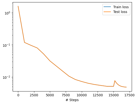
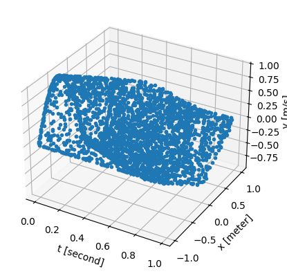
Let’s visualize and save the data.
trainer.saveplot(issave=True, isplot=True)
Saving loss history to D:\codes\projects\pinnx\docs\examples-pinn-forward\loss.dat ...
Saving checkpoint into D:\codes\projects\pinnx\docs\examples-pinn-forward\loss.dat
Saving training data to D:\codes\projects\pinnx\docs\examples-pinn-forward\train.dat ...
Saving checkpoint into D:\codes\projects\pinnx\docs\examples-pinn-forward\train.dat
Saving test data to D:\codes\projects\pinnx\docs\examples-pinn-forward\test.dat ...
Saving checkpoint into D:\codes\projects\pinnx\docs\examples-pinn-forward\test.dat
We can also test the model with the data:
def gen_testdata():
    data = np.load("../dataset/Burgers.npz")
    t, x, exact = data["t"], data["x"], data["usol"].T
    xx, tt = np.meshgrid(x, t)
    X = {'x': np.ravel(xx) * u.meter, 't': np.ravel(tt) * u.second}
    y = exact.flatten()[:, None]
    return X, y * uy
X, y_true = gen_testdata()
y_pred = trainer.predict(X)
f = pde(X, y_pred)
print("Mean residual:", u.math.mean(u.math.absolute(f)))
print("L2 relative error:", pinnx.metrics.l2_relative_error(y_true, y_pred['y']))
Mean residual: 0.02894243 * (meter / second) / second
L2 relative error: 224.70277