
Inverse problem for the Poisson equation with unknown forcing field#
Problem setup#
We will solve
with the Dirichlet boundary conditions
Here, both \(u(x)\) and \(q(x)\) are unknown. Furthermore, we have the measurement of \(u(x)\) at 100 points.
The reference solution is \(u(x) = \sin(\pi x), \quad q(x) = -\pi^2 \sin(\pi x)\).
Dimensional analysis#
Assumptions on dimensions:
Let \([x] = L\), where \(L\) represents length.
Let \([u] = U\), where \(U\) represents the dimension of the unknown field \(u\). For instance, \(u\) could represent displacement, temperature, potential, etc. The exact choice of \(U\) depends on the physical context.
The dimension of \(q(x)\) is to be determined.
Dimensional Analysis:
Consider the left-hand side (LHS): \(\frac{d^2 u}{dx^2}\) Its dimension is:
\[ \left[\frac{d^2 u}{dx^2}\right] = \frac{[u]}{[x]^2} = \frac{U}{L^2}. \]For the equation to be dimensionally consistent, the right-hand side (RHS) \(q(x)\) must have the same dimension as the LHS: $\( [q(x)] = \frac{U}{L^2}. \)$
Summary:
If the dimension of \(u\) is \(U\) and the dimension of \(x\) is \(L\), then the source term \(q(x)\) must have the dimension \(U/L^2\).
In other words, the source term \(q(x)\) is the field quantity \(u\) per unit length squared. The physical meaning depends on the specific problem. For example, if \(u\) represents temperature, then \(q(x)\) might represent a thermal energy source density. If \(u\) represents an electric potential, then \(q(x)\) may relate to charge distribution (scaled appropriately by physical constants).
Implementation#
Import the necessary package:
import brainstate
import brainunit as u
import matplotlib.pyplot as plt
import numpy as np

import pinnx
Define the units for the problem:
unit_of_x = u.meter
unit_of_u = u.newton
unit_of_q = u.newton / unit_of_x ** 2
Define the problem.
def pde(x, y):
    du_xx = net.hessian(x, y='u')['u']['x']['x']
    return -du_xx + y['q']


geom = pinnx.geometry.Interval(-1, 1).to_dict_point(x=unit_of_x)
Define the Dirichlet boundary conditions.
def sol(x):
    # solution is u(x) = sin(pi*x), q(x) = -pi^2 * sin(pi*x)
    # return {'u': u.math.sin(u.math.pi * x['x']), }
    return {
        'u': u.math.sin(u.math.pi * x['x'] / unit_of_x) * unit_of_u,
        'q': -u.math.pi ** 2 * u.math.sin(u.math.pi * x['x'] / unit_of_x) * unit_of_q
    }


bc = pinnx.icbc.DirichletBC(sol)
Define the observation points and the training data generator.
def gen_traindata(num):
    # generate num equally-spaced points from -1 to 1
    xvals = np.linspace(-1, 1, num)
    uvals = np.sin(np.pi * xvals)
    return {'x': xvals * unit_of_x}, {'u': uvals * unit_of_u}


ob_x, ob_u = gen_traindata(100)
observe_u = pinnx.icbc.PointSetBC(ob_x, ob_u)
Define the neural network model, adding the unit information to the input and output:
net = pinnx.nn.Model(
    pinnx.nn.DictToArray(x=unit_of_x),
    pinnx.nn.PFNN([1, [20, 20], [20, 20], [20, 20], 2], "tanh", braintools.init.KaimingUniform()),
    pinnx.nn.ArrayToDict(u=unit_of_u, q=unit_of_q),
)
The final problem:
problem = pinnx.problem.PDE(
    geom,
    pde,
    [bc, observe_u],
    net,
    num_domain=200,
    num_boundary=2,
    anchors=ob_x,
    num_test=1000,
    loss_weights=[1, 100, 1000],
)
Train the model:
model = pinnx.Trainer(problem)
model.compile(braintools.optim.Adam(0.0001)).train(iterations=20000)
model.saveplot(issave=True, isplot=True)
Compiling trainer...
'compile' took 0.049581 s

Training trainer...

Step      Train loss                                     Test loss                                      Test metric
0         [57.104668 * pascal2,                          [58.55549 * pascal2,                           []
           {'ibc0': {'q': 71.43462 * pascal,              {'ibc0': {'q': 71.43462 * pascal,
                     'u': 21.93853 * newton}},                      'u': 21.93853 * newton}},
           {'ibc1': {'u': 1383.2239 * newton}}]           {'ibc1': {'u': 1383.2239 * newton}}]
1000      [9.099975 * pascal2,                           [9.277513 * pascal2,                           []
           {'ibc0': {'q': 0.02584232 * pascal,            {'ibc0': {'q': 0.02584232 * pascal,
                     'u': 39.094223 * newton}},                     'u': 39.094223 * newton}},
           {'ibc1': {'u': 89.13055 * newton}}]            {'ibc1': {'u': 89.13055 * newton}}]
2000      [17.813923 * pascal2,                          [17.973166 * pascal2,                          []
           {'ibc0': {'q': 0.03595128 * pascal,            {'ibc0': {'q': 0.03595128 * pascal,
                     'u': 22.458023 * newton}},                     'u': 22.458023 * newton}},
           {'ibc1': {'u': 49.399963 * newton}}]           {'ibc1': {'u': 49.399963 * newton}}]
3000      [20.421053 * pascal2,                          [20.553577 * pascal2,                          []
           {'ibc0': {'q': 0.03406093 * pascal,            {'ibc0': {'q': 0.03406093 * pascal,
                     'u': 12.548685 * newton}},                     'u': 12.548685 * newton}},
           {'ibc1': {'u': 26.532593 * newton}}]           {'ibc1': {'u': 26.532593 * newton}}]
4000      [18.949293 * pascal2,                          [19.105434 * pascal2,                          []
           {'ibc0': {'q': 0.03712923 * pascal,            {'ibc0': {'q': 0.03712923 * pascal,
                     'u': 6.2132597 * newton}},                     'u': 6.2132597 * newton}},
           {'ibc1': {'u': 12.868485 * newton}}]           {'ibc1': {'u': 12.868485 * newton}}]
5000      [15.683843 * pascal2,                          [15.849516 * pascal2,                          []
           {'ibc0': {'q': 0.03507624 * pascal,            {'ibc0': {'q': 0.03507624 * pascal,
                     'u': 2.9483395 * newton}},                     'u': 2.9483395 * newton}},
           {'ibc1': {'u': 6.0103345 * newton}}]           {'ibc1': {'u': 6.0103345 * newton}}]
6000      [11.3106 * pascal2,                            [11.44179 * pascal2,                           []
           {'ibc0': {'q': 0.02415182 * pascal,            {'ibc0': {'q': 0.02415182 * pascal,
                     'u': 1.4232403 * newton}},                     'u': 1.4232403 * newton}},
           {'ibc1': {'u': 2.9394844 * newton}}]           {'ibc1': {'u': 2.9394844 * newton}}]
7000      [6.889275 * pascal2,                           [6.9675927 * pascal2,                          []
           {'ibc0': {'q': 0.01458644 * pascal,            {'ibc0': {'q': 0.01458644 * pascal,
                     'u': 0.7137065 * newton}},                     'u': 0.7137065 * newton}},
           {'ibc1': {'u': 1.5752933 * newton}}]           {'ibc1': {'u': 1.5752933 * newton}}]
8000      [3.0519495 * pascal2,                          [3.085175 * pascal2,                           []
           {'ibc0': {'q': 0.00667563 * pascal,            {'ibc0': {'q': 0.00667563 * pascal,
                     'u': 0.33465862 * newton}},                    'u': 0.33465862 * newton}},
           {'ibc1': {'u': 0.84809256 * newton}}]          {'ibc1': {'u': 0.84809256 * newton}}]
9000      [1.0699911 * pascal2,                          [1.0805568 * pascal2,                          []
           {'ibc0': {'q': 0.0019603 * pascal,             {'ibc0': {'q': 0.0019603 * pascal,
                     'u': 0.14555798 * newton}},                    'u': 0.14555798 * newton}},
           {'ibc1': {'u': 0.529897 * newton}}]            {'ibc1': {'u': 0.529897 * newton}}]
10000     [0.36260056 * pascal2,                         [0.36515456 * pascal2,                         []
           {'ibc0': {'q': 0.00053385 * pascal,            {'ibc0': {'q': 0.00053385 * pascal,
                     'u': 0.06022839 * newton}},                    'u': 0.06022839 * newton}},
           {'ibc1': {'u': 0.4085685 * newton}}]           {'ibc1': {'u': 0.4085685 * newton}}]
11000     [0.18483813 * pascal2,                         [0.1858395 * pascal2,                          []
           {'ibc0': {'q': 0.00012002 * pascal,            {'ibc0': {'q': 0.00012002 * pascal,
                     'u': 0.02717585 * newton}},                    'u': 0.02717585 * newton}},
           {'ibc1': {'u': 0.3386068 * newton}}]           {'ibc1': {'u': 0.3386068 * newton}}]
12000     [0.12419797 * pascal2,                         [0.12520623 * pascal2,                         []
           {'ibc0': {'q': 6.49303e-05 * pascal,           {'ibc0': {'q': 6.49303e-05 * pascal,
                     'u': 0.01508655 * newton}},                    'u': 0.01508655 * newton}},
           {'ibc1': {'u': 0.252522 * newton}}]            {'ibc1': {'u': 0.252522 * newton}}]
13000     [0.07476345 * pascal2,                         [0.07559747 * pascal2,                         []
           {'ibc0': {'q': 0.00022872 * pascal,            {'ibc0': {'q': 0.00022872 * pascal,
                     'u': 0.00766858 * newton}},                    'u': 0.00766858 * newton}},
           {'ibc1': {'u': 0.15152633 * newton}}]          {'ibc1': {'u': 0.15152633 * newton}}]
14000     [0.0346879 * pascal2,                          [0.0351154 * pascal2,                          []
           {'ibc0': {'q': 1.1295616e-05 * pascal,         {'ibc0': {'q': 1.1295616e-05 * pascal,
                     'u': 0.00236588 * newton}},                    'u': 0.00236588 * newton}},
           {'ibc1': {'u': 0.07225788 * newton}}]          {'ibc1': {'u': 0.07225788 * newton}}]
15000     [0.01340395 * pascal2,                         [0.01357405 * pascal2,                         []
           {'ibc0': {'q': 5.2584824e-06 * pascal,         {'ibc0': {'q': 5.2584824e-06 * pascal,
                     'u': 0.00018877 * newton}},                    'u': 0.00018877 * newton}},
           {'ibc1': {'u': 0.03148581 * newton}}]          {'ibc1': {'u': 0.03148581 * newton}}]
16000     [0.00504076 * pascal2,                         [0.00508512 * pascal2,                         []
           {'ibc0': {'q': 2.1729034e-05 * pascal,         {'ibc0': {'q': 2.1729034e-05 * pascal,
                     'u': 3.5908473e-05 * newton}},                 'u': 3.5908473e-05 * newton}},
           {'ibc1': {'u': 0.01453501 * newton}}]          {'ibc1': {'u': 0.01453501 * newton}}]
17000     [0.00211953 * pascal2,                         [0.00213015 * pascal2,                         []
           {'ibc0': {'q': 3.1532704e-06 * pascal,         {'ibc0': {'q': 3.1532704e-06 * pascal,
                     'u': 0.00025964 * newton}},                    'u': 0.00025964 * newton}},
           {'ibc1': {'u': 0.00791687 * newton}}]          {'ibc1': {'u': 0.00791687 * newton}}]
18000     [0.0009769 * pascal2,                          [0.00098521 * pascal2,                         []
           {'ibc0': {'q': 3.8374005e-06 * pascal,         {'ibc0': {'q': 3.8374005e-06 * pascal,
                     'u': 0.00030924 * newton}},                    'u': 0.00030924 * newton}},
           {'ibc1': {'u': 0.00499536 * newton}}]          {'ibc1': {'u': 0.00499536 * newton}}]
19000     [0.00052247 * pascal2,                         [0.00052762 * pascal2,                         []
           {'ibc0': {'q': 3.1709257e-07 * pascal,         {'ibc0': {'q': 3.1709257e-07 * pascal,
                     'u': 0.00027461 * newton}},                    'u': 0.00027461 * newton}},
           {'ibc1': {'u': 0.00339381 * newton}}]          {'ibc1': {'u': 0.00339381 * newton}}]
20000     [0.00034573 * pascal2,                         [0.00034509 * pascal2,                         []
           {'ibc0': {'q': 8.5156114e-07 * pascal,         {'ibc0': {'q': 8.5156114e-07 * pascal,
                     'u': 0.00021139 * newton}},                    'u': 0.00021139 * newton}},
           {'ibc1': {'u': 0.00248489 * newton}}]          {'ibc1': {'u': 0.00248489 * newton}}]

Best trainer at step 20000:
  train loss: 3.04e-03
  test loss: 3.04e-03
  test metric: []

'train' took 42.773905 s

Saving loss history to D:\codes\projects\pinnx\docs\examples-pinn-inverse\loss.dat ...
Saving checkpoint into D:\codes\projects\pinnx\docs\examples-pinn-inverse\loss.dat
Saving training data to D:\codes\projects\pinnx\docs\examples-pinn-inverse\train.dat ...
Saving checkpoint into D:\codes\projects\pinnx\docs\examples-pinn-inverse\train.dat
Saving test data to D:\codes\projects\pinnx\docs\examples-pinn-inverse\test.dat ...
Saving checkpoint into D:\codes\projects\pinnx\docs\examples-pinn-inverse\test.dat


Visualize the results:
# view results
x = geom.uniform_points(500)
yhat = model.predict(x)
uhat = yhat['u'] / unit_of_u
qhat = yhat['q'] / unit_of_q
x = x['x'] / unit_of_x
utrue = np.sin(np.pi * x)
print("l2 relative error for u: " + str(pinnx.metrics.l2_relative_error(utrue, uhat)))
plt.figure()
plt.plot(x, utrue, "-", label="u_true")
plt.plot(x, uhat, "--", label="u_NN")
plt.legend()
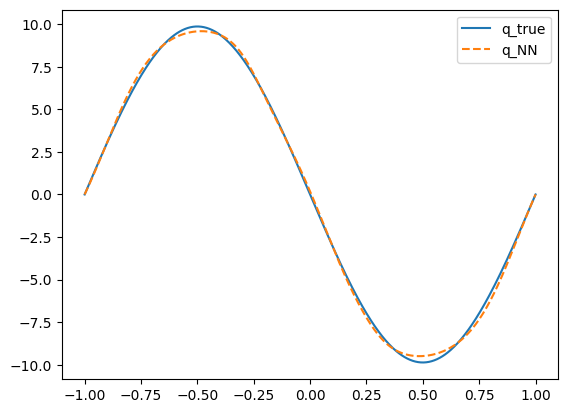
qtrue = -np.pi ** 2 * np.sin(np.pi * x)
print("l2 relative error for q: " + str(pinnx.metrics.l2_relative_error(qtrue, qhat)))
plt.figure()
plt.plot(x, qtrue, "-", label="q_true")
plt.plot(x, qhat, "--", label="q_NN")
plt.legend()
plt.show()
l2 relative error for u: 0.0022317795
l2 relative error for q: 0.02959022

Complete code please see the code in elliptic_inverse_field.py.