Laplace equation on a disk#
Problem setup#
We will solve a Laplace equation in a polar coordinate system:
with the Dirichlet boundary condition
and the periodic boundary condition
The reference solution is \(y=r\cos(\theta)\).
Dimensional Analysis for the Laplace Equation on a Disk#
Problem Setup#
We will solve the Laplace equation in a polar coordinate system:
with the Dirichlet boundary condition:
and the periodic boundary condition:
The reference solution is:
Dimensional Analysis#
Step 1: Assign Dimensions to Variables#
Radial Coordinate \(r\):
The dimension of \(r\) is length:
\[ [r] = L. \]
Angular Coordinate \(\theta\):
The dimension of \(\theta\) is dimensionless:
\[ [\theta] = 1. \]
Solution \(y\):
The solution \(y\) represents a physical quantity, which we assume to be in volts (V):
\[ [y] = V. \]
Step 2: Analyze the Dimensions of Each Term#
First Derivative Term \(r\frac{dy}{dr}\):
The first derivative \(\frac{dy}{dr}\) has dimensions:
\[ \left[\frac{dy}{dr}\right] = \frac{[y]}{[r]} = \frac{V}{L}. \]Therefore, the term \(r\frac{dy}{dr}\) has dimensions:
\[ \left[r\frac{dy}{dr}\right] = [r] \cdot \frac{V}{L} = L \cdot \frac{V}{L} = V. \]
Second Derivative Term \(r^2\frac{d^2y}{dr^2}\):
The second derivative \(\frac{d^2y}{dr^2}\) has dimensions:
\[ \left[\frac{d^2y}{dr^2}\right] = \frac{[y]}{[r]^2} = \frac{V}{L^2}. \]Therefore, the term \(r^2\frac{d^2y}{dr^2}\) has dimensions:
\[ \left[r^2\frac{d^2y}{dr^2}\right] = [r]^2 \cdot \frac{V}{L^2} = L^2 \cdot \frac{V}{L^2} = V. \]
Second Derivative Term \(\frac{d^2y}{d\theta^2}\):
The second derivative \(\frac{d^2y}{d\theta^2}\) has dimensions:
\[ \left[\frac{d^2y}{d\theta^2}\right] = \frac{[y]}{[\theta]^2} = \frac{V}{1^2} = V. \]
Step 3: Verify Dimensional Consistency#
The Laplace equation in polar coordinates is:
Each term in the equation has dimensions of \(V\):
\(r\frac{dy}{dr}\): \(V\)
\(r^2\frac{d^2y}{dr^2}\): \(V\)
\(\frac{d^2y}{d\theta^2}\): \(V\)
Since all terms have the same dimensions, the equation is dimensionally consistent.
Step 4: Summary of Dimensions#
Variable/Parameter |
Physical Meaning |
Dimensions |
|---|---|---|
\(r\) |
Radial coordinate |
\(L\) |
\(\theta\) |
Angular coordinate |
\(1\) (dimensionless) |
\(y\) |
Solution (e.g., voltage) |
\(V\) |
Step 5: Initial and Boundary Conditions#
Boundary Condition \(y(1,\theta) = \cos(\theta)\):
The boundary condition \(y(1,\theta) = \cos(\theta)\) is given in volts:
\[ [y(1,\theta)] = V. \]The term \(\cos(\theta)\) is dimensionless because \(\theta\) is dimensionless.
Periodic Boundary Condition \(y(r, \theta + 2\pi) = y(r, \theta)\):
The periodic boundary condition ensures that the solution is periodic in \(\theta\) with period \(2\pi\).
Since \(\theta\) is dimensionless, the condition is dimensionally consistent.
Implementation#
This description goes through the implementation of a solver for the above described Heat equation step-by-step.
First, import the libraries we need:
import braintools
import brainunit as u
import numpy as np

import pinnx
We begin by defining a computational geometry. We can use a built-in class Rectangle as follows
geom = pinnx.geometry.Rectangle(
    xmin=[0, 0],
    xmax=[1, 2 * np.pi],
).to_dict_point(r=u.meter, theta=u.radian)
Next, we express the PDE residual of the Laplace equation:
def pde(x, y):
    jacobian = net.jacobian(x)
    hessian = net.hessian(x)

    dy_r = jacobian["y"]["r"]
    dy_rr = hessian["y"]["r"]["r"]
    dy_thetatheta = hessian["y"]["theta"]["theta"]
    return x['r'] * dy_r + x['r'] ** 2 * dy_rr + dy_thetatheta
The first argument to pde is 2-dimensional vector where the first component(x[:,0:1]) is \(r\)-coordinate and the second componenet (x[:,1:]) is the \(\theta\)-coordinate. The second argument is the network output, i.e., the solution \(y(r, \theta)\).
Next, we consider the Dirichlet boundary condition. We need to implement a function, which should return True for points inside the subdomain and False for the points outside. In our case, if the points satisfy \(r=1\) and are on the whole boundary of the rectangle domain, then function boundary returns True. Otherwise, it returns False. (Note that because of rounding-off errors, it is often wise to use u.math.allclose to test whether two floating point values are equivalent.)
def boundary(x, on_boundary):
    return on_boundary and u.math.allclose(x['r'], 1)
The argument x to boundary is the network input and is a \(d\)-dim vector, where \(d\) is the dimension and \(d=2\) in this case. To facilitate the implementation of boundary, a boolean on_boundary is used as the second argument. If the point \(r,\theta\) (the first argument) is on the entire boundary of the rectangle geometry that created above, then on_boundary is True, otherwise, on_boundary is False.
Using a lambda funtion, the boundary we defined above can be passed to DirichletBC as the second argument. Thus, the Dirichlet boundary condition is
uy = u.volt / u.meter
bc = pinnx.icbc.DirichletBC(
    lambda x: {'y': u.math.cos(x['theta']) * uy},
    lambda x, on_boundary: u.math.logical_and(on_boundary, u.math.allclose(x['r'], 1 * u.meter)),
)
If we rewrite this problem in cartesian coordinates, the variables are in the form of \([r\sin(\theta), r\cos(\theta)]\). We use them as features to satisfy the certain underlying physical constraints, so that the network is automatically periodic along the \(\theta\) coordinate and the period is \(2\pi\).
Next, we choose the network. Here, we use a fully connected neural network of depth 4 (i.e., 3 hidden layers) and width 20:
# Use [r*sin(theta), r*cos(theta)] as features,
# so that the network is automatically periodic along the theta coordinate.
def feature_transform(x):
    x = pinnx.utils.array_to_dict(x, ["r", "theta"], keep_dim=True)
    return u.math.concatenate([x['r'] * u.math.sin(x['theta']),
                               x['r'] * u.math.cos(x['theta'])], axis=-1)

net = pinnx.nn.Model(
    pinnx.nn.DictToArray(r=u.meter, theta=u.radian),
    pinnx.nn.FNN([2] + [20] * 3 + [1], "tanh", input_transform=feature_transform),
    pinnx.nn.ArrayToDict(y=uy),
)
Now, we have specified the geometry, PDE residual, and boundary condition. We then define the PDE problem as
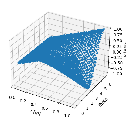
The argument solution is the reference solution to compute the error of our solution, and we define it as follows:
def solution(x):
    r, theta = x['r'], x['theta']
    return {'y': r * u.math.cos(theta) * uy / u.meter}
problem = pinnx.problem.PDE(
    geom,
    pde,
    bc,
    net,
    num_domain=2540,
    num_boundary=80,
    solution=solution
)
Now, we have the PDE problem and the network. We bulid a trainer and choose the optimizer and learning rate:
trainer = pinnx.Trainer(problem)
trainer.compile(braintools.optim.Adam(1e-3), metrics=["l2 relative error"])
Compiling trainer...
'compile' took 0.093740 s
<pinnx.Trainer at 0x141369fd0>
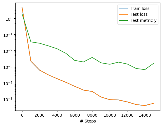
We then train the model for 15000 iterations:
trainer.train(iterations=15000)
Training trainer...

Step      Train loss                                                            Test loss                                                             Test metric
0         [3.4136772 * 10.0^0 * (meter * (volt / meter) / meter) ** 2,          [3.4136772 * 10.0^0 * (meter * (volt / meter) / meter) ** 2,          [{'y': Array(1.9016247, dtype=float32)}]
           {'ibc0': {'y': 1.2442183 * volt / meter}}]                            {'ibc0': {'y': 1.2442183 * volt / meter}}]
1000      [0.00209501 * 10.0^0 * (meter * (volt / meter) / meter) ** 2,         [0.00209501 * 10.0^0 * (meter * (volt / meter) / meter) ** 2,         [{'y': Array(0.03482116, dtype=float32)}]
           {'ibc0': {'y': 9.6204014e-05 * volt / meter}}]                        {'ibc0': {'y': 9.6204014e-05 * volt / meter}}]
2000      [0.00059394 * 10.0^0 * (meter * (volt / meter) / meter) ** 2,         [0.00059394 * 10.0^0 * (meter * (volt / meter) / meter) ** 2,         [{'y': Array(0.02848322, dtype=float32)}]
           {'ibc0': {'y': 1.8821578e-05 * volt / meter}}]                        {'ibc0': {'y': 1.8821578e-05 * volt / meter}}]
3000      [0.0003004 * 10.0^0 * (meter * (volt / meter) / meter) ** 2,          [0.0003004 * 10.0^0 * (meter * (volt / meter) / meter) ** 2,          [{'y': Array(0.01964555, dtype=float32)}]
           {'ibc0': {'y': 1.1315266e-05 * volt / meter}}]                        {'ibc0': {'y': 1.1315266e-05 * volt / meter}}]
4000      [0.0001739 * 10.0^0 * (meter * (volt / meter) / meter) ** 2,          [0.0001739 * 10.0^0 * (meter * (volt / meter) / meter) ** 2,          [{'y': Array(0.0129396, dtype=float32)}]
           {'ibc0': {'y': 8.526638e-06 * volt / meter}}]                         {'ibc0': {'y': 8.526638e-06 * volt / meter}}]
5000      [0.00010057 * 10.0^0 * (meter * (volt / meter) / meter) ** 2,         [0.00010057 * 10.0^0 * (meter * (volt / meter) / meter) ** 2,         [{'y': Array(0.00673189, dtype=float32)}]
           {'ibc0': {'y': 6.3102784e-06 * volt / meter}}]                        {'ibc0': {'y': 6.3102784e-06 * volt / meter}}]
6000      [5.6971734e-05 * 10.0^0 * (meter * (volt / meter) / meter) ** 2,      [5.6971734e-05 * 10.0^0 * (meter * (volt / meter) / meter) ** 2,      [{'y': Array(0.00247048, dtype=float32)}]
           {'ibc0': {'y': 4.33217e-06 * volt / meter}}]                          {'ibc0': {'y': 4.33217e-06 * volt / meter}}]
7000      [3.255158e-05 * 10.0^0 * (meter * (volt / meter) / meter) ** 2,       [3.255158e-05 * 10.0^0 * (meter * (volt / meter) / meter) ** 2,       [{'y': Array(0.0019735, dtype=float32)}]
           {'ibc0': {'y': 2.83005e-06 * volt / meter}}]                          {'ibc0': {'y': 2.83005e-06 * volt / meter}}]
8000      [2.4938374e-05 * 10.0^0 * (meter * (volt / meter) / meter) ** 2,      [2.4938374e-05 * 10.0^0 * (meter * (volt / meter) / meter) ** 2,      [{'y': Array(0.00377944, dtype=float32)}]
           {'ibc0': {'y': 4.333744e-06 * volt / meter}}]                         {'ibc0': {'y': 4.333744e-06 * volt / meter}}]
9000      [1.1950426e-05 * 10.0^0 * (meter * (volt / meter) / meter) ** 2,      [1.1950426e-05 * 10.0^0 * (meter * (volt / meter) / meter) ** 2,      [{'y': Array(0.00174527, dtype=float32)}]
           {'ibc0': {'y': 1.2896384e-06 * volt / meter}}]                        {'ibc0': {'y': 1.2896384e-06 * volt / meter}}]
10000     [8.125793e-06 * 10.0^0 * (meter * (volt / meter) / meter) ** 2,       [8.125793e-06 * 10.0^0 * (meter * (volt / meter) / meter) ** 2,       [{'y': Array(0.00141424, dtype=float32)}]
           {'ibc0': {'y': 9.607884e-07 * volt / meter}}]                         {'ibc0': {'y': 9.607884e-07 * volt / meter}}]
11000     [7.288996e-06 * 10.0^0 * (meter * (volt / meter) / meter) ** 2,       [7.288996e-06 * 10.0^0 * (meter * (volt / meter) / meter) ** 2,       [{'y': Array(0.00191965, dtype=float32)}]
           {'ibc0': {'y': 1.3772864e-06 * volt / meter}}]                        {'ibc0': {'y': 1.3772864e-06 * volt / meter}}]
12000     [5.566375e-06 * 10.0^0 * (meter * (volt / meter) / meter) ** 2,       [5.566375e-06 * 10.0^0 * (meter * (volt / meter) / meter) ** 2,       [{'y': Array(0.00146894, dtype=float32)}]
           {'ibc0': {'y': 9.980397e-07 * volt / meter}}]                         {'ibc0': {'y': 9.980397e-07 * volt / meter}}]
13000     [4.0166346e-06 * 10.0^0 * (meter * (volt / meter) / meter) ** 2,      [4.0166346e-06 * 10.0^0 * (meter * (volt / meter) / meter) ** 2,      [{'y': Array(0.00078307, dtype=float32)}]
           {'ibc0': {'y': 4.9924233e-07 * volt / meter}}]                        {'ibc0': {'y': 4.9924233e-07 * volt / meter}}]
14000     [3.4733355e-06 * 10.0^0 * (meter * (volt / meter) / meter) ** 2,      [3.4733355e-06 * 10.0^0 * (meter * (volt / meter) / meter) ** 2,      [{'y': Array(0.00065782, dtype=float32)}]
           {'ibc0': {'y': 4.2479667e-07 * volt / meter}}]                        {'ibc0': {'y': 4.2479667e-07 * volt / meter}}]
15000     [4.31375e-06 * 10.0^0 * (meter * (volt / meter) / meter) ** 2,        [4.31375e-06 * 10.0^0 * (meter * (volt / meter) / meter) ** 2,        [{'y': Array(0.0016097, dtype=float32)}]
           {'ibc0': {'y': 1.0574405e-06 * volt / meter}}]                        {'ibc0': {'y': 1.0574405e-06 * volt / meter}}]

Best trainer at step 14000:
  train loss: 3.90e-06
  test loss: 3.90e-06
  test metric: [{'y': Array(0., dtype=float32)}]

'train' took 56.701270 s
<pinnx.Trainer at 0x141369fd0>
We also save and plot the best trained result and loss history.
trainer.saveplot(issave=True, isplot=True)
Saving loss history to /Users/sichaohe/Documents/GitHub/pinnx/docs/examples-pinn-forward/loss.dat ...
Saving checkpoint into /Users/sichaohe/Documents/GitHub/pinnx/docs/examples-pinn-forward/loss.dat
Saving training data to /Users/sichaohe/Documents/GitHub/pinnx/docs/examples-pinn-forward/train.dat ...
Saving checkpoint into /Users/sichaohe/Documents/GitHub/pinnx/docs/examples-pinn-forward/train.dat
Saving test data to /Users/sichaohe/Documents/GitHub/pinnx/docs/examples-pinn-forward/test.dat ...
Saving checkpoint into /Users/sichaohe/Documents/GitHub/pinnx/docs/examples-pinn-forward/test.dat