
Inferring the effective viscosity and permeability for the Brinkman-Forchheimer model#
The problem we need to solve#
The Brinkman-Forchheimer model can be viewed as an extended Darcy’s law and is used to describe wall-bounded porous media flows:
where the solution \(u\) is the fluid velocity, \(g\) denotes the external force, \(\nu\) is the kinetic viscosity of fluid, \(\epsilon\) is the porosity of the porous medium, and \(K\) is the permeability. The effective viscosity, \(\nu_e\), is related to the pore structure and hardly to be determined. A no-slip boundary condition is imposed, i.e., \(u(0)=u(1)=0.\) The analytic solution for this problem is
with \(r=\sqrt{\nu\epsilon/\nu_eK}.\) We choose \(H=1,\nu_e=\nu=10^{-3},\epsilon=0.4\), and \(K=10^{-3}\), and \(g=1.\) To infer \(\nu_e\),we collect the data measurements of the velocity \(u\) in only 5 sensor locations.
Dimensional analysis#
Variables and Parameters:
Spatial Coordinate, \(x\)
Typical dimension: length \([x] = L\).
Fluid Velocity, \(u(x)\)
Velocity dimension: \([u] = L/T\).
Kinematic Viscosity of the Fluid, \(\nu\)
Kinematic viscosity has dimensions: \([\nu] = L^2/T\).
Effective Viscosity, \(\nu_e\)
This is also a (generalized) viscosity term, so it has the same dimension as kinematic viscosity: \([\nu_e] = L^2/T\).
Porosity, \(\epsilon\)
Porosity is a dimensionless measure of void fraction: \([\epsilon] = 1\) (no units).
Permeability, \(K\)
Permeability has dimensions of area: \([K] = L^2\).
External Force, \(g\)
The right-hand side \(g\) must match the dimensions of the left-hand side terms.
Consider the term \(-\frac{\nu_e}{\epsilon}\nabla^2 u\): \(\nabla^2 u \sim u/L^2 = (L/T)/L^2 = 1/(T L)\). Multiplying by \(\nu_e = L^2/T\) yields \((L^2/T)*(1/(T L)) = L/T^2\).
Similarly, \(\frac{\nu u}{K} = (L^2/T)*(L/T)/(L^2) = L/T^2\).
Thus both terms on the left-hand side have dimension \(L/T^2\).
Hence, \([g] = L/T^2\).
Summarized Dimensions:
\([x] = L\)
\([u] = L/T\)
\([\nu] = L^2/T\)
\([\nu_e] = L^2/T\)
\([\epsilon] = 1\) (dimensionless)
\([K] = L^2\)
\([g] = L/T^2\)
\([H] = L\)
Given values (with dimensions):
\(H=1\,L\)
\(\nu_e=10^{-3}\,L^2/T\)
\(\nu=10^{-3}\,L^2/T\)
\(\epsilon=0.4\,(\text{dimensionless})\)
\(K=10^{-3}\,L^2\)
\(g=1\,L/T^2\)
All chosen parameters are dimensionally consistent with the governing equation.
Implementation#
Import the package we need:
import brainstate
import braintools
import brainunit as u
import numpy as np

import pinnx
Define the parameters with physical units and the analytical solution:
g = 1 * u.meter / u.second ** 2
v = 1e-3 * u.meter ** 2 / u.second
e = 0.4
H = 1 * u.meter

v_e = brainstate.ParamState(0.1 * u.meter ** 2 / u.second)
K = brainstate.ParamState(0.001 * u.meter ** 2)


def sol(x):
    x = x['x'].mantissa
    r = (v.mantissa * e / (1e-3 * 1e-3)) ** 0.5
    y = (
        g.mantissa * 1e-3 /
        v.mantissa *
        (1 - u.math.cosh(r * (x - H.mantissa / 2)) /
         u.math.cosh(r * H.mantissa / 2))
    )
    return {'y': y * u.meter / u.second}
Define the geometry of the problem:
geom = pinnx.geometry.Interval(0, 1).to_dict_point(x=u.meter)
Define the PDE and generate training data:
def pde(x, y):
    du_xx = net.hessian(x)["y"]["x"]["x"]
    return -v_e.value / e * du_xx + v * y['y'] / K.value - g
def gen_traindata(num):
    xvals = np.linspace(1 / (num + 1), 1, num, endpoint=False)
    x = {'x': xvals * u.meter}
    return x, sol(x)

ob_x, ob_u = gen_traindata(5)
observe_u = pinnx.icbc.PointSetBC(ob_x, ob_u)
Define the neural network model:
net = pinnx.nn.Model(
    pinnx.nn.DictToArray(x=u.meter),
    pinnx.nn.FNN(
        [1] + [20] * 3 + [1], "tanh",
        output_transform=lambda x, y: x * (1 - x) * y
    ),
    pinnx.nn.ArrayToDict(y=u.meter / u.second),
)
Define the problem and solve it:
problem = pinnx.problem.PDE(
    geom,
    pde,
    approximator=net,
    solution=sol,
    constraints=[observe_u],
    num_domain=100,
    num_boundary=0,
    train_distribution="uniform",
    num_test=500,
)
Train the model:
variable = pinnx.callbacks.VariableValue([v_e, K], period=200, filename="../examples-pinn-inverse/variables1.dat")
trainer = pinnx.Trainer(problem, external_trainable_variables=[v_e, K])
trainer.compile(braintools.optim.Adam(0.001), metrics=["l2 relative error"]).train(iterations=30000, callbacks=[variable])
trainer.saveplot(issave=True, isplot=True)
Compiling trainer...
'compile' took 0.066302 s
Training trainer...
Step Train loss Test loss Test metric
0 [1.2322745 * 10.0^0 * metre ** 2 * second ** -4, [1.2312626 * 10.0^0 * metre ** 2 * second ** -4, [{'y': Array(1.0370464, dtype=float32)}]
{'ibc0': {'y': 1.0472959 * meter / second}}] {'ibc0': {'y': 1.0472959 * meter / second}}]
1000 [0.00070408 * 10.0^0 * metre ** 2 * second ** -4, [0.00077674 * 10.0^0 * metre ** 2 * second ** -4, [{'y': Array(0.26238587, dtype=float32)}]
{'ibc0': {'y': 0.0429582 * meter / second}}] {'ibc0': {'y': 0.0429582 * meter / second}}]
2000 [0.00269285 * 10.0^0 * metre ** 2 * second ** -4, [0.00285477 * 10.0^0 * metre ** 2 * second ** -4, [{'y': Array(0.24537273, dtype=float32)}]
{'ibc0': {'y': 0.03586509 * meter / second}}] {'ibc0': {'y': 0.03586509 * meter / second}}]
3000 [0.00576497 * 10.0^0 * metre ** 2 * second ** -4, [0.00623961 * 10.0^0 * metre ** 2 * second ** -4, [{'y': Array(0.20437899, dtype=float32)}]
{'ibc0': {'y': 0.02151751 * meter / second}}] {'ibc0': {'y': 0.02151751 * meter / second}}]
4000 [0.00459755 * 10.0^0 * metre ** 2 * second ** -4, [0.00526482 * 10.0^0 * metre ** 2 * second ** -4, [{'y': Array(0.15171465, dtype=float32)}]
{'ibc0': {'y': 0.0091022 * meter / second}}] {'ibc0': {'y': 0.0091022 * meter / second}}]
5000 [0.00277259 * 10.0^0 * metre ** 2 * second ** -4, [0.0033845 * 10.0^0 * metre ** 2 * second ** -4, [{'y': Array(0.11733841, dtype=float32)}]
{'ibc0': {'y': 0.00427992 * meter / second}}] {'ibc0': {'y': 0.00427992 * meter / second}}]
6000 [0.00165531 * 10.0^0 * metre ** 2 * second ** -4, [0.00217546 * 10.0^0 * metre ** 2 * second ** -4, [{'y': Array(0.09476856, dtype=float32)}]
{'ibc0': {'y': 0.00225442 * meter / second}}] {'ibc0': {'y': 0.00225442 * meter / second}}]
7000 [0.00104619 * 10.0^0 * metre ** 2 * second ** -4, [0.00148209 * 10.0^0 * metre ** 2 * second ** -4, [{'y': Array(0.07885406, dtype=float32)}]
{'ibc0': {'y': 0.00126963 * meter / second}}] {'ibc0': {'y': 0.00126963 * meter / second}}]
8000 [0.00072733 * 10.0^0 * metre ** 2 * second ** -4, [0.00110027 * 10.0^0 * metre ** 2 * second ** -4, [{'y': Array(0.06720789, dtype=float32)}]
{'ibc0': {'y': 0.00075283 * meter / second}}] {'ibc0': {'y': 0.00075283 * meter / second}}]
9000 [0.00063628 * 10.0^0 * metre ** 2 * second ** -4, [0.00099117 * 10.0^0 * metre ** 2 * second ** -4, [{'y': Array(0.05862389, dtype=float32)}]
{'ibc0': {'y': 0.00049126 * meter / second}}] {'ibc0': {'y': 0.00049126 * meter / second}}]
10000 [0.00038361 * 10.0^0 * metre ** 2 * second ** -4, [0.00070372 * 10.0^0 * metre ** 2 * second ** -4, [{'y': Array(0.05175733, dtype=float32)}]
{'ibc0': {'y': 0.00034356 * meter / second}}] {'ibc0': {'y': 0.00034356 * meter / second}}]
11000 [0.00030018 * 10.0^0 * metre ** 2 * second ** -4, [0.00058416 * 10.0^0 * metre ** 2 * second ** -4, [{'y': Array(0.04615347, dtype=float32)}]
{'ibc0': {'y': 0.00025155 * meter / second}}] {'ibc0': {'y': 0.00025155 * meter / second}}]
12000 [0.00021172 * 10.0^0 * metre ** 2 * second ** -4, [0.00048861 * 10.0^0 * metre ** 2 * second ** -4, [{'y': Array(0.04148087, dtype=float32)}]
{'ibc0': {'y': 0.00018796 * meter / second}}] {'ibc0': {'y': 0.00018796 * meter / second}}]
13000 [0.00019228 * 10.0^0 * metre ** 2 * second ** -4, [0.00044553 * 10.0^0 * metre ** 2 * second ** -4, [{'y': Array(0.03766144, dtype=float32)}]
{'ibc0': {'y': 0.00014382 * meter / second}}] {'ibc0': {'y': 0.00014382 * meter / second}}]
14000 [0.00017108 * 10.0^0 * metre ** 2 * second ** -4, [0.00044543 * 10.0^0 * metre ** 2 * second ** -4, [{'y': Array(0.0341393, dtype=float32)}]
{'ibc0': {'y': 0.00010903 * meter / second}}] {'ibc0': {'y': 0.00010903 * meter / second}}]
15000 [0.00013393 * 10.0^0 * metre ** 2 * second ** -4, [0.00039608 * 10.0^0 * metre ** 2 * second ** -4, [{'y': Array(0.03076173, dtype=float32)}]
{'ibc0': {'y': 8.177792e-05 * meter / second}}] {'ibc0': {'y': 8.177792e-05 * meter / second}}]
16000 [8.0808204e-05 * 10.0^0 * metre ** 2 * second ** -4, [0.0003569 * 10.0^0 * metre ** 2 * second ** -4, [{'y': Array(0.02793985, dtype=float32)}]
{'ibc0': {'y': 6.29709e-05 * meter / second}}] {'ibc0': {'y': 6.29709e-05 * meter / second}}]
17000 [0.00011505 * 10.0^0 * metre ** 2 * second ** -4, [0.00042251 * 10.0^0 * metre ** 2 * second ** -4, [{'y': Array(0.0253933, dtype=float32)}]
{'ibc0': {'y': 4.9956318e-05 * meter / second}}] {'ibc0': {'y': 4.9956318e-05 * meter / second}}]
18000 [9.197639e-05 * 10.0^0 * metre ** 2 * second ** -4, [0.00039912 * 10.0^0 * metre ** 2 * second ** -4, [{'y': Array(0.02277111, dtype=float32)}]
{'ibc0': {'y': 3.684857e-05 * meter / second}}] {'ibc0': {'y': 3.684857e-05 * meter / second}}]
19000 [0.0010154 * 10.0^0 * metre ** 2 * second ** -4, [0.00129051 * 10.0^0 * metre ** 2 * second ** -4, [{'y': Array(0.02021311, dtype=float32)}]
{'ibc0': {'y': 3.3709657e-05 * meter / second}}] {'ibc0': {'y': 3.3709657e-05 * meter / second}}]
20000 [5.1668612e-05 * 10.0^0 * metre ** 2 * second ** -4, [0.00041443 * 10.0^0 * metre ** 2 * second ** -4, [{'y': Array(0.01882938, dtype=float32)}]
{'ibc0': {'y': 2.288534e-05 * meter / second}}] {'ibc0': {'y': 2.288534e-05 * meter / second}}]
21000 [3.3456847e-05 * 10.0^0 * metre ** 2 * second ** -4, [0.00041545 * 10.0^0 * metre ** 2 * second ** -4, [{'y': Array(0.0172698, dtype=float32)}]
{'ibc0': {'y': 1.875132e-05 * meter / second}}] {'ibc0': {'y': 1.875132e-05 * meter / second}}]
22000 [5.7533292e-05 * 10.0^0 * metre ** 2 * second ** -4, [0.00046078 * 10.0^0 * metre ** 2 * second ** -4, [{'y': Array(0.01577936, dtype=float32)}]
{'ibc0': {'y': 1.50083115e-05 * meter / second}}] {'ibc0': {'y': 1.50083115e-05 * meter / second}}]
23000 [2.343095e-05 * 10.0^0 * metre ** 2 * second ** -4, [0.00048284 * 10.0^0 * metre ** 2 * second ** -4, [{'y': Array(0.01447075, dtype=float32)}]
{'ibc0': {'y': 1.2138024e-05 * meter / second}}] {'ibc0': {'y': 1.2138024e-05 * meter / second}}]
24000 [1.470709e-05 * 10.0^0 * metre ** 2 * second ** -4, [0.00047367 * 10.0^0 * metre ** 2 * second ** -4, [{'y': Array(0.01338609, dtype=float32)}]
{'ibc0': {'y': 1.0363932e-05 * meter / second}}] {'ibc0': {'y': 1.0363932e-05 * meter / second}}]
25000 [0.00023094 * 10.0^0 * metre ** 2 * second ** -4, [0.00074617 * 10.0^0 * metre ** 2 * second ** -4, [{'y': Array(0.01255435, dtype=float32)}]
{'ibc0': {'y': 9.4853285e-06 * meter / second}}] {'ibc0': {'y': 9.4853285e-06 * meter / second}}]
26000 [1.3408353e-05 * 10.0^0 * metre ** 2 * second ** -4, [0.00052996 * 10.0^0 * metre ** 2 * second ** -4, [{'y': Array(0.01138956, dtype=float32)}]
{'ibc0': {'y': 7.0691417e-06 * meter / second}}] {'ibc0': {'y': 7.0691417e-06 * meter / second}}]
27000 [2.6520533e-05 * 10.0^0 * metre ** 2 * second ** -4, [0.00054236 * 10.0^0 * metre ** 2 * second ** -4, [{'y': Array(0.01050647, dtype=float32)}]
{'ibc0': {'y': 5.9204394e-06 * meter / second}}] {'ibc0': {'y': 5.9204394e-06 * meter / second}}]
28000 [1.0871769e-05 * 10.0^0 * metre ** 2 * second ** -4, [0.00052523 * 10.0^0 * metre ** 2 * second ** -4, [{'y': Array(0.00997761, dtype=float32)}]
{'ibc0': {'y': 5.3106005e-06 * meter / second}}] {'ibc0': {'y': 5.3106005e-06 * meter / second}}]
29000 [5.7753732e-05 * 10.0^0 * metre ** 2 * second ** -4, [0.00058264 * 10.0^0 * metre ** 2 * second ** -4, [{'y': Array(0.00915718, dtype=float32)}]
{'ibc0': {'y': 4.4464914e-06 * meter / second}}] {'ibc0': {'y': 4.4464914e-06 * meter / second}}]
30000 [1.193763e-05 * 10.0^0 * metre ** 2 * second ** -4, [0.00057735 * 10.0^0 * metre ** 2 * second ** -4, [{'y': Array(0.00868338, dtype=float32)}]
{'ibc0': {'y': 3.8816847e-06 * meter / second}}] {'ibc0': {'y': 3.8816847e-06 * meter / second}}]
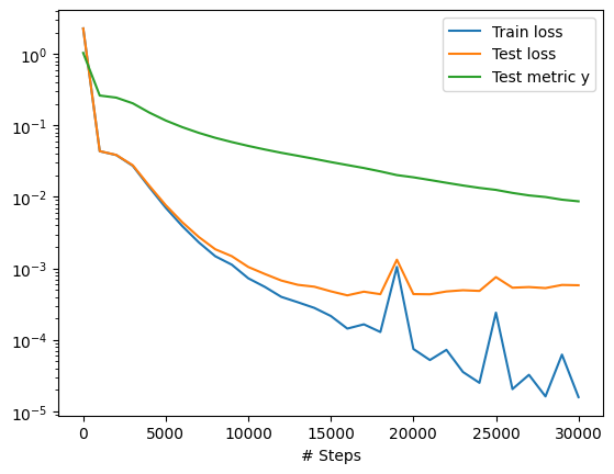
Best trainer at step 30000:
train loss: 1.58e-05
test loss: 5.81e-04
test metric: [{'y': Array(0.01, dtype=float32)}]
'train' took 14.610238 s
Saving loss history to D:\codes\projects\pinnx\docs\examples-pinn-inverse\loss.dat ...
Saving checkpoint into D:\codes\projects\pinnx\docs\examples-pinn-inverse\loss.dat
Saving training data to D:\codes\projects\pinnx\docs\examples-pinn-inverse\train.dat ...
Saving checkpoint into D:\codes\projects\pinnx\docs\examples-pinn-inverse\train.dat
Saving test data to D:\codes\projects\pinnx\docs\examples-pinn-inverse\test.dat ...
Saving checkpoint into D:\codes\projects\pinnx\docs\examples-pinn-inverse\test.dat
The complete code is available in the Brinkman-Forchheimer model example.