Heat equation#
Problem setup#
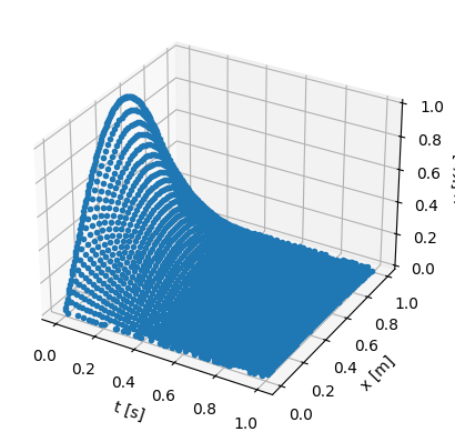
We will solve a heat equation:
where \(alpha=0.4\) is the thermal diffusivity constant.
With Dirichlet boundary conditions:
and periodic(sinusoidal) inital condition:
where \(L=1\) is the length of the bar, \(n=1\) is the frequency of the sinusoidal initial conditions.
The exact solution is \(u(x,t) = e^{\frac{-n ^2\pi ^2 \alpha t}{L^2}}\sin (\frac{n\pi x}{L})\).
Dimensional Analysis#
Step 1: Assign Dimensions to Variables#
Spatial Coordinate \(x\):
The dimension of \(x\) is length:
\[ [x] = L. \]
Time \(t\):
The dimension of time is:
\[ [t] = T. \]
Temperature \(u\):
Temperature has dimensions of temperature:
\[ [u] = \Theta. \]
Thermal Diffusivity \(\alpha\):
The term \(\alpha \frac{\partial^2 u}{\partial x^2}\) involves the second spatial derivative of temperature, which must have the same dimensions as the time derivative \(\frac{\partial u}{\partial t}\).
Step 2: Analyze the Dimensions of Each Term#
Time Derivative Term:
The time derivative \(\frac{\partial u}{\partial t}\) has dimensions:
\[ \left[\frac{\partial u}{\partial t}\right] = \frac{[u]}{[t]} = \frac{\Theta}{T}. \]
Diffusion Term:
The diffusion term \(\alpha \frac{\partial^2 u}{\partial x^2}\) involves the second spatial derivative of temperature:
\[ \left[\frac{\partial^2 u}{\partial x^2}\right] = \frac{[u]}{[x]^2} = \frac{\Theta}{L^2}. \]Therefore, the diffusion term has dimensions:
\[ \left[\alpha \frac{\partial^2 u}{\partial x^2}\right] = [\alpha] \cdot \frac{\Theta}{L^2} = \frac{\Theta}{T}. \]
Step 3: Determine the Dimensions of \(\alpha\)#
The diffusion term \(\alpha \frac{\partial^2 u}{\partial x^2}\) must have the same dimensions as the time derivative \(\frac{\partial u}{\partial t}\):
\[ [\alpha] \cdot \frac{\Theta}{L^2} = \frac{\Theta}{T} \implies [\alpha] = \frac{L^2}{T}. \]Therefore, the thermal diffusivity \(\alpha\) has dimensions of thermal diffusivity:
\[ [\alpha] = \frac{L^2}{T}. \]
Step 4: Summary of Dimensions#
Variable/Parameter |
Physical Meaning |
Dimensions |
|---|---|---|
\(x\) |
Spatial coordinate |
\(L\) |
\(t\) |
Time |
\(T\) |
\(u\) |
Temperature |
\(\Theta\) |
\(\alpha\) |
Thermal diffusivity |
\(L^2 / T\) |
Step 5: Initial and Boundary Conditions#
Boundary Conditions:
The boundary conditions \(u(0,t) = u(1,t) = 0\) are given in temperature units:
\[ [u(0,t)] = [u(1,t)] = \Theta. \]
Initial Condition:
The initial condition \(u(x,0) = \sin \left(\frac{n\pi x}{L}\right)\) is given in temperature units:
\[ [u(x,0)] = \Theta. \]The term \(\sin \left(\frac{n\pi x}{L}\right)\) is dimensionless because \(\frac{n\pi x}{L}\) is dimensionless (\(n\) and \(\pi\) are dimensionless constants, and \(x\) and \(L\) have the same dimensions).
Implementation#
This description goes through the implementation of a solver for the above described Heat equation step-by-step.
First, import the libraries we need:
import brainstate
import braintools
import optax
import brainunit as u

import pinnx
We begin by defining the parameters of the equation:
a = 0.4 * u.meter2 / u.second # Thermal diffusivity
L = 1 * u.meter  # Length of the bar
n = 1 * u.Hz # Frequency of the sinusoidal initial conditions
Next, we define a computational geometry and time domain. We can use a built-in class Interval and TimeDomain and we combine both the domains using GeometryXTime as follows
geomtime = pinnx.geometry.GeometryXTime(
    geometry=pinnx.geometry.Interval(0., 1.),
    timedomain=pinnx.geometry.TimeDomain(0., 1.)
).to_dict_point(x=u.meter, t=u.second)
Next, we express the PDE residual of the Heat equation:
@brainstate.transform.jit
def pde(x, y):
    jacobian = approximator.jacobian(x)
    hessian = approximator.hessian(x)
    dy_t = jacobian['y']['t']
    dy_xx = hessian['y']['x']['x']
    return dy_t - a * dy_xx
The first argument to pde is 2-dimensional vector where the first component(x[:,0]) is x-coordinate and the second componenet (x[:,1]) is the t-coordinate. The second argument is the network output, i.e., the solution u(x,t), but here we use y as the name of the variable.
Next, we consider the boundary/initial condition. We include the geomtime space, time geometry created above. We also define IC which is the inital condition for the burgers equation and we use the computational domain and initial function.
uy = u.kelvin / u.second
# Initial and boundary conditions:
bc = pinnx.icbc.DirichletBC(
    lambda x : {'y': 0. * uy}
)
ic = pinnx.icbc.IC(
    lambda x: {'y': u.math.sin(n * u.math.pi * x['x'] / L, unit_to_scale=u.becquerel) * uy},
)
Next, we choose the network. Here, we use a fully connected neural network of depth 4 (i.e., 3 hidden layers) and width 20:
approximator = pinnx.nn.Model(
    pinnx.nn.DictToArray(x=u.meter, t=u.second),
    pinnx.nn.FNN(
        [2] + [20] * 3 + [1],
        "tanh",
        braintools.init.KaimingUniform()
    ),
    pinnx.nn.ArrayToDict(y=uy)
)
Now, we have specified the geometry, PDE residual, boundary/initial condition and approximator. We then define the TimePDE problem as
problem = pinnx.problem.TimePDE(
    geomtime,
    pde,
    [bc, ic],
    approximator,
    num_domain=2540,
    num_boundary=80,
    num_initial=160,
    num_test=2540,
)
Warning: 2540 points required, but 2550 points sampled.
The number 2540 is the number of training residual points sampled inside the domain, and the number 80 is the number of training points sampled on the boundary. We also include 160 initial residual points for the initial conditions.
Now, we have the PDE problem and the network. We build a Model and choose the optimizer and learning rate:
trainer = pinnx.Trainer(problem)
trainer.compile(braintools.optim.Adam(1e-3))
Compiling trainer...
'compile' took 0.057718 s
<pinnx.Trainer at 0x140369fd0>
We then train the model for 10000 iterations:
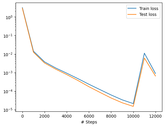
trainer.train(iterations=10000)
Training trainer...

Step      Train loss                                                        Test loss                                                         Test metric
0         [1.7518853 * 10.0^0 * ((kelvin / second) / second) ** 2,          [1.5275408 * 10.0^0 * ((kelvin / second) / second) ** 2,          []
           {'ibc0': {'y': 0.32626745 * kelvin / second}},                    {'ibc0': {'y': 0.32626745 * kelvin / second}},
           {'ibc1': {'y': 1.0854373 * kelvin / second}}]                     {'ibc1': {'y': 1.0854373 * kelvin / second}}]
1000      [0.00440458 * 10.0^0 * ((kelvin / second) / second) ** 2,         [0.00259006 * 10.0^0 * ((kelvin / second) / second) ** 2,         []
           {'ibc0': {'y': 0.00315431 * kelvin / second}},                    {'ibc0': {'y': 0.00315431 * kelvin / second}},
           {'ibc1': {'y': 0.0065606 * kelvin / second}}]                     {'ibc1': {'y': 0.0065606 * kelvin / second}}]
2000      [0.00167008 * 10.0^0 * ((kelvin / second) / second) ** 2,         [0.00116817 * 10.0^0 * ((kelvin / second) / second) ** 2,         []
           {'ibc0': {'y': 0.00121897 * kelvin / second}},                    {'ibc0': {'y': 0.00121897 * kelvin / second}},
           {'ibc1': {'y': 0.00086062 * kelvin / second}}]                    {'ibc1': {'y': 0.00086062 * kelvin / second}}]
3000      [0.00081106 * 10.0^0 * ((kelvin / second) / second) ** 2,         [0.00056661 * 10.0^0 * ((kelvin / second) / second) ** 2,         []
           {'ibc0': {'y': 0.00062208 * kelvin / second}},                    {'ibc0': {'y': 0.00062208 * kelvin / second}},
           {'ibc1': {'y': 0.00032557 * kelvin / second}}]                    {'ibc1': {'y': 0.00032557 * kelvin / second}}]
4000      [0.00046928 * 10.0^0 * ((kelvin / second) / second) ** 2,         [0.000322 * 10.0^0 * ((kelvin / second) / second) ** 2,           []
           {'ibc0': {'y': 0.00029971 * kelvin / second}},                    {'ibc0': {'y': 0.00029971 * kelvin / second}},
           {'ibc1': {'y': 0.00014895 * kelvin / second}}]                    {'ibc1': {'y': 0.00014895 * kelvin / second}}]
5000      [0.00028848 * 10.0^0 * ((kelvin / second) / second) ** 2,         [0.00019277 * 10.0^0 * ((kelvin / second) / second) ** 2,         []
           {'ibc0': {'y': 0.00011767 * kelvin / second}},                    {'ibc0': {'y': 0.00011767 * kelvin / second}},
           {'ibc1': {'y': 6.189949e-05 * kelvin / second}}]                  {'ibc1': {'y': 6.189949e-05 * kelvin / second}}]
6000      [0.00018016 * 10.0^0 * ((kelvin / second) / second) ** 2,         [0.00011896 * 10.0^0 * ((kelvin / second) / second) ** 2,         []
           {'ibc0': {'y': 3.331493e-05 * kelvin / second}},                  {'ibc0': {'y': 3.331493e-05 * kelvin / second}},
           {'ibc1': {'y': 1.836832e-05 * kelvin / second}}]                  {'ibc1': {'y': 1.836832e-05 * kelvin / second}}]
7000      [0.00010137 * 10.0^0 * ((kelvin / second) / second) ** 2,         [6.64615e-05 * 10.0^0 * ((kelvin / second) / second) ** 2,        []
           {'ibc0': {'y': 1.1578003e-05 * kelvin / second}},                 {'ibc0': {'y': 1.1578003e-05 * kelvin / second}},
           {'ibc1': {'y': 6.0143293e-06 * kelvin / second}}]                 {'ibc1': {'y': 6.0143293e-06 * kelvin / second}}]
8000      [5.2904743e-05 * 10.0^0 * ((kelvin / second) / second) ** 2,      [3.3663386e-05 * 10.0^0 * ((kelvin / second) / second) ** 2,      []
           {'ibc0': {'y': 5.493999e-06 * kelvin / second}},                  {'ibc0': {'y': 5.493999e-06 * kelvin / second}},
           {'ibc1': {'y': 2.8610739e-06 * kelvin / second}}]                 {'ibc1': {'y': 2.8610739e-06 * kelvin / second}}]
9000      [2.8543282e-05 * 10.0^0 * ((kelvin / second) / second) ** 2,      [1.8309089e-05 * 10.0^0 * ((kelvin / second) / second) ** 2,      []
           {'ibc0': {'y': 3.213987e-06 * kelvin / second}},                  {'ibc0': {'y': 3.213987e-06 * kelvin / second}},
           {'ibc1': {'y': 1.6611314e-06 * kelvin / second}}]                 {'ibc1': {'y': 1.6611314e-06 * kelvin / second}}]
10000     [1.7808488e-05 * 10.0^0 * ((kelvin / second) / second) ** 2,      [1.16582605e-05 * 10.0^0 * ((kelvin / second) / second) ** 2,     []
           {'ibc0': {'y': 2.0270465e-06 * kelvin / second}},                 {'ibc0': {'y': 2.0270465e-06 * kelvin / second}},
           {'ibc1': {'y': 1.0902334e-06 * kelvin / second}}]                 {'ibc1': {'y': 1.0902334e-06 * kelvin / second}}]

Best trainer at step 10000:
  train loss: 2.09e-05
  test loss: 1.48e-05
  test metric: []

'train' took 47.118451 s
<pinnx.Trainer at 0x140369fd0>
After we train the network using Adam, we continue to train the network using L-BFGS to achieve a smaller loss:
trainer.compile(braintools.optim.OptaxOptimizer(optax.lbfgs(1e-3, linesearch=None)))
trainer.train(iterations=2000)
Compiling trainer...
'compile' took 0.128015 s

Training trainer...

Step      Train loss                                                            Test loss                                                              Test metric
10000     [1.7808488e-05 * 10.0^0 * ((kelvin / second) / second) ** 2,          [1.16582605e-05 * 10.0^0 * ((kelvin / second) / second) ** 2,          []
           {'ibc0': {'y': 2.0270465e-06 * kelvin / second}},                     {'ibc0': {'y': 2.0270465e-06 * kelvin / second}},
           {'ibc1': {'y': 1.0902334e-06 * kelvin / second}}]                     {'ibc1': {'y': 1.0902334e-06 * kelvin / second}}]
11000     [0.00920797 * 10.0^0 * ((kelvin / second) / second) ** 2,             [0.00422679 * 10.0^0 * ((kelvin / second) / second) ** 2,              []
           {'ibc0': {'y': 0.00172434 * kelvin / second}},                        {'ibc0': {'y': 0.00172434 * kelvin / second}},
           {'ibc1': {'y': 6.910529e-05 * kelvin / second}}]                      {'ibc1': {'y': 6.910529e-05 * kelvin / second}}]
12000     [0.0007039 * 10.0^0 * ((kelvin / second) / second) ** 2,              [0.00046745 * 10.0^0 * ((kelvin / second) / second) ** 2,              []
           {'ibc0': {'y': 0.00013835 * kelvin / second}},                        {'ibc0': {'y': 0.00013835 * kelvin / second}},
           {'ibc1': {'y': 3.9120117e-05 * kelvin / second}}]                     {'ibc1': {'y': 3.9120117e-05 * kelvin / second}}]

Best trainer at step 10000:
  train loss: 2.09e-05
  test loss: 1.48e-05
  test metric: []

'train' took 10.107104 s
<pinnx.Trainer at 0x140369fd0>
Let’s visualize and save the data.
trainer.saveplot(issave=True, isplot=True)
Saving loss history to /Users/sichaohe/Documents/GitHub/pinnx/docs/examples-pinn-forward/loss.dat ...
Saving checkpoint into /Users/sichaohe/Documents/GitHub/pinnx/docs/examples-pinn-forward/loss.dat
Saving training data to /Users/sichaohe/Documents/GitHub/pinnx/docs/examples-pinn-forward/train.dat ...
Saving checkpoint into /Users/sichaohe/Documents/GitHub/pinnx/docs/examples-pinn-forward/train.dat
Saving test data to /Users/sichaohe/Documents/GitHub/pinnx/docs/examples-pinn-forward/test.dat ...
Saving checkpoint into /Users/sichaohe/Documents/GitHub/pinnx/docs/examples-pinn-forward/test.dat