Inferring the space-dependent reaction rate in a diffusion-reaction system#
The problem we need to solve#
We consider a one-dimensional diffusion-reaction system in which the reaction rate \(k(x)\) is a space-dependent function:
where \(\lambda=0.01\) is the diffusion coefficient, \(u\) is the solute concentration, and \(f=\sin(2\pi x)\) is the source term. The objective is to infer \(k(x)\) given measurements on \(u.\) The exact unknown reaction rate is
In addition, the condition \(u(x)=0\) is imposed at \(x=0\) and 1.
Dimensional analysis#
Below is a dimensional analysis for each variable and parameter in the given one-dimensional diffusion-reaction equation:
Governing equation: $\( \lambda \frac{\partial^2 u}{\partial x^2} - k(x)u = f, \quad x \in [0,1]. \)$
Physical meanings and typical dimensions:
Spatial coordinate, \( x \)
Typically, a spatial coordinate has the dimension of length:
\[ [x] = L. \]
Solute concentration, \( u(x) \)
Concentration is commonly expressed as mass per unit volume (assuming a mass-based concentration):
\[ [u] = M / L^3. \]
Diffusion coefficient, \( \lambda \)
A diffusion coefficient typically has dimensions of length squared per time:
\[ [\lambda] = L^2 / T. \]
Reaction rate, \( k(x) \)
Consider the term \( k(x)u \). This must have the same dimension as \(\lambda \frac{\partial^2 u}{\partial x^2}\).
The Laplacian term \(\frac{\partial^2 u}{\partial x^2}\) has dimension \((M/L^3) / L^2 = M / (L^5)\).
Multiplying by \(\lambda = L^2/T\) gives \((L^2/T)*(M/L^5) = M/(T L^3)\).
Therefore, \(k(x)u\) must also have dimension \(M/(T L^3)\). Given \( [u] = M/L^3 \), it follows:
\[ [k(x)] [u] = M/(T L^3) \implies [k(x)] (M/L^3) = M/(T L^3) \implies [k(x)] = 1/T. \]
Thus, the reaction rate \(k(x)\) has units of inverse time, which makes sense physically.
Source term, \( f \)
The source term \( f \) appears on the right-hand side of the equation and must have the same dimension as the left-hand side terms. We have already found that \(\lambda \frac{\partial^2 u}{\partial x^2}\) and \(k(x)u\) both have dimensions \( M/(T L^3) \). Hence:
\[ [f] = M/(T L^3). \]
Summary of Dimensions:
\([x] = L\)
\([u] = M/L^3\)
\([\lambda] = L^2/T\)
\([k(x)] = 1/T\)
\([f] = M/(T L^3)\)
These dimensions are consistent with a diffusion-reaction system where:
\(u\) is a concentration (mass per volume),
\(\lambda\) is a diffusion coefficient (length²/time),
\(k(x)\) is a reaction rate (1/time),
\(f\) is a source term with the dimension of a generation/consumption rate of mass per volume per time.
Implementation#
First, import the necessary libraries:
import brainstate
import brainunit as u
import matplotlib.pyplot as plt
import numpy as np
from scipy.integrate import solve_bvp

import pinnx
Define the units for the variables and parameters:
unit_of_x = u.meter
unit_of_u = u.mole / u.meter ** 3
unit_of_f = u.mole / (u.second * u.meter ** 3)

l = 0.01 * unit_of_x ** 2 / u.second
Define the solution for the solute concentration:
def k(x):
    return 0.1 + np.exp(-0.5 * (x - 0.5) ** 2 / 0.15 ** 2)


def fun(x, y):
    return np.vstack((y[1], (k(x) * y[0] + np.sin(2 * np.pi * x)) / l.mantissa))


def bc(ya, yb):
    return np.array([ya[0], yb[0]])


num = 100
xvals = np.linspace(0, 1, num)
y = np.zeros((2, xvals.size))
res = solve_bvp(fun, bc, xvals, y)
Define the PDE for the neural network model:
geom = pinnx.geometry.Interval(0, 1).to_dict_point(x=unit_of_x)


def pde(x, y):
    hessian = net.hessian(x, y='u')
    du_xx = hessian["u"]["x"]["x"]
    f = u.math.sin(2 * np.pi * x['x'].mantissa) * unit_of_f
    return l * du_xx - y['u'] * y['k'] - f
Define the neural network model:
net = pinnx.nn.Model(
    pinnx.nn.DictToArray(x=unit_of_x),
    pinnx.nn.PFNN([1, [20, 20], [20, 20], 2], "tanh", braintools.init.KaimingUniform()),
    pinnx.nn.ArrayToDict(u=unit_of_u, k=1 / u.second),
)
Define the training data:
def gen_traindata():
    x = {'x': xvals * unit_of_x}
    y = {'u': res.sol(xvals)[0] * unit_of_u}
    return x, y


ob_x, ob_u = gen_traindata()
observe_u = pinnx.icbc.PointSetBC(ob_x, ob_u)
Define the boundary conditions:
bc = pinnx.icbc.DirichletBC(lambda x: {'u': 0 * unit_of_u})
Define the PDE problem:
problem = pinnx.problem.PDE(
    geom,
    pde,
    constraints=[bc, observe_u],
    approximator=net,
    num_domain=50,
    num_boundary=8,
    train_distribution="uniform",
    num_test=1000,
)
Train the model:
model = pinnx.Trainer(problem)
model.compile(braintools.optim.Adam(1e-3)).train(iterations=20000)
Compiling trainer...
'compile' took 0.046593 s

Training trainer...

Step      Train loss                                                                         Test loss                                                                          Test metric
0         [0.42841953 * 10.0^0 * (meter2 / second * (mmolar / meter) / meter) ** 2,          [0.48738545 * 10.0^0 * (meter2 / second * (mmolar / meter) / meter) ** 2,          []
           {'ibc0': {'u': 0.04377487 * mmolar}},                                              {'ibc0': {'u': 0.04377487 * mmolar}},
           {'ibc1': {'u': 0.76479465 * mmolar}}]                                              {'ibc1': {'u': 0.76479465 * mmolar}}]
1000      [0.00161212 * 10.0^0 * (meter2 / second * (mmolar / meter) / meter) ** 2,          [0.00137106 * 10.0^0 * (meter2 / second * (mmolar / meter) / meter) ** 2,          []
           {'ibc0': {'u': 0.00100709 * mmolar}},                                              {'ibc0': {'u': 0.00100709 * mmolar}},
           {'ibc1': {'u': 0.0077876 * mmolar}}]                                               {'ibc1': {'u': 0.0077876 * mmolar}}]
2000      [0.00086259 * 10.0^0 * (meter2 / second * (mmolar / meter) / meter) ** 2,          [0.00051533 * 10.0^0 * (meter2 / second * (mmolar / meter) / meter) ** 2,          []
           {'ibc0': {'u': 4.4753404e-05 * mmolar}},                                           {'ibc0': {'u': 4.4753404e-05 * mmolar}},
           {'ibc1': {'u': 0.00127289 * mmolar}}]                                              {'ibc1': {'u': 0.00127289 * mmolar}}]
3000      [0.00062482 * 10.0^0 * (meter2 / second * (mmolar / meter) / meter) ** 2,          [0.00038163 * 10.0^0 * (meter2 / second * (mmolar / meter) / meter) ** 2,          []
           {'ibc0': {'u': 1.1394843e-05 * mmolar}},                                           {'ibc0': {'u': 1.1394843e-05 * mmolar}},
           {'ibc1': {'u': 0.00050347 * mmolar}}]                                              {'ibc1': {'u': 0.00050347 * mmolar}}]
4000      [0.00029539 * 10.0^0 * (meter2 / second * (mmolar / meter) / meter) ** 2,          [0.00020541 * 10.0^0 * (meter2 / second * (mmolar / meter) / meter) ** 2,          []
           {'ibc0': {'u': 1.0836469e-06 * mmolar}},                                           {'ibc0': {'u': 1.0836469e-06 * mmolar}},
           {'ibc1': {'u': 0.0001564 * mmolar}}]                                               {'ibc1': {'u': 0.0001564 * mmolar}}]
5000      [0.00010554 * 10.0^0 * (meter2 / second * (mmolar / meter) / meter) ** 2,          [8.63514e-05 * 10.0^0 * (meter2 / second * (mmolar / meter) / meter) ** 2,         []
           {'ibc0': {'u': 5.5338234e-08 * mmolar}},                                           {'ibc0': {'u': 5.5338234e-08 * mmolar}},
           {'ibc1': {'u': 4.1387873e-05 * mmolar}}]                                           {'ibc1': {'u': 4.1387873e-05 * mmolar}}]
6000      [3.261345e-05 * 10.0^0 * (meter2 / second * (mmolar / meter) / meter) ** 2,        [3.0046363e-05 * 10.0^0 * (meter2 / second * (mmolar / meter) / meter) ** 2,       []
           {'ibc0': {'u': 4.189261e-08 * mmolar}},                                            {'ibc0': {'u': 4.189261e-08 * mmolar}},
           {'ibc1': {'u': 1.1832751e-05 * mmolar}}]                                           {'ibc1': {'u': 1.1832751e-05 * mmolar}}]
7000      [1.0917592e-05 * 10.0^0 * (meter2 / second * (mmolar / meter) / meter) ** 2,       [1.06402085e-05 * 10.0^0 * (meter2 / second * (mmolar / meter) / meter) ** 2,      []
           {'ibc0': {'u': 6.6463612e-09 * mmolar}},                                           {'ibc0': {'u': 6.6463612e-09 * mmolar}},
           {'ibc1': {'u': 3.1595891e-06 * mmolar}}]                                           {'ibc1': {'u': 3.1595891e-06 * mmolar}}]
8000      [5.7016923e-06 * 10.0^0 * (meter2 / second * (mmolar / meter) / meter) ** 2,       [5.549621e-06 * 10.0^0 * (meter2 / second * (mmolar / meter) / meter) ** 2,        []
           {'ibc0': {'u': 1.4118614e-06 * mmolar}},                                           {'ibc0': {'u': 1.4118614e-06 * mmolar}},
           {'ibc1': {'u': 2.000358e-06 * mmolar}}]                                            {'ibc1': {'u': 2.000358e-06 * mmolar}}]
9000      [3.0069625e-06 * 10.0^0 * (meter2 / second * (mmolar / meter) / meter) ** 2,       [2.992862e-06 * 10.0^0 * (meter2 / second * (mmolar / meter) / meter) ** 2,        []
           {'ibc0': {'u': 6.584769e-09 * mmolar}},                                            {'ibc0': {'u': 6.584769e-09 * mmolar}},
           {'ibc1': {'u': 5.5307254e-07 * mmolar}}]                                           {'ibc1': {'u': 5.5307254e-07 * mmolar}}]
10000     [2.0530574e-06 * 10.0^0 * (meter2 / second * (mmolar / meter) / meter) ** 2,       [2.0282348e-06 * 10.0^0 * (meter2 / second * (mmolar / meter) / meter) ** 2,       []
           {'ibc0': {'u': 1.3601655e-08 * mmolar}},                                           {'ibc0': {'u': 1.3601655e-08 * mmolar}},
           {'ibc1': {'u': 5.196718e-07 * mmolar}}]                                            {'ibc1': {'u': 5.196718e-07 * mmolar}}]
11000     [1.5368364e-06 * 10.0^0 * (meter2 / second * (mmolar / meter) / meter) ** 2,       [1.4977886e-06 * 10.0^0 * (meter2 / second * (mmolar / meter) / meter) ** 2,       []
           {'ibc0': {'u': 8.276815e-08 * mmolar}},                                            {'ibc0': {'u': 8.276815e-08 * mmolar}},
           {'ibc1': {'u': 5.301843e-07 * mmolar}}]                                            {'ibc1': {'u': 5.301843e-07 * mmolar}}]
12000     [1.1885431e-06 * 10.0^0 * (meter2 / second * (mmolar / meter) / meter) ** 2,       [1.1730367e-06 * 10.0^0 * (meter2 / second * (mmolar / meter) / meter) ** 2,       []
           {'ibc0': {'u': 1.5201218e-08 * mmolar}},                                           {'ibc0': {'u': 1.5201218e-08 * mmolar}},
           {'ibc1': {'u': 5.8795325e-07 * mmolar}}]                                           {'ibc1': {'u': 5.8795325e-07 * mmolar}}]
13000     [9.736607e-07 * 10.0^0 * (meter2 / second * (mmolar / meter) / meter) ** 2,        [9.640654e-07 * 10.0^0 * (meter2 / second * (mmolar / meter) / meter) ** 2,        []
           {'ibc0': {'u': 1.3303917e-08 * mmolar}},                                           {'ibc0': {'u': 1.3303917e-08 * mmolar}},
           {'ibc1': {'u': 6.254742e-07 * mmolar}}]                                            {'ibc1': {'u': 6.254742e-07 * mmolar}}]
14000     [8.2432285e-07 * 10.0^0 * (meter2 / second * (mmolar / meter) / meter) ** 2,       [8.188007e-07 * 10.0^0 * (meter2 / second * (mmolar / meter) / meter) ** 2,        []
           {'ibc0': {'u': 1.3247805e-08 * mmolar}},                                           {'ibc0': {'u': 1.3247805e-08 * mmolar}},
           {'ibc1': {'u': 6.5696383e-07 * mmolar}}]                                           {'ibc1': {'u': 6.5696383e-07 * mmolar}}]
15000     [6.123539e-06 * 10.0^0 * (meter2 / second * (mmolar / meter) / meter) ** 2,        [6.9687558e-06 * 10.0^0 * (meter2 / second * (mmolar / meter) / meter) ** 2,       []
           {'ibc0': {'u': 8.313561e-06 * mmolar}},                                            {'ibc0': {'u': 8.313561e-06 * mmolar}},
           {'ibc1': {'u': 8.073111e-06 * mmolar}}]                                            {'ibc1': {'u': 8.073111e-06 * mmolar}}]
16000     [6.50423e-07 * 10.0^0 * (meter2 / second * (mmolar / meter) / meter) ** 2,         [6.7078685e-07 * 10.0^0 * (meter2 / second * (mmolar / meter) / meter) ** 2,       []
           {'ibc0': {'u': 8.236504e-08 * mmolar}},                                            {'ibc0': {'u': 8.236504e-08 * mmolar}},
           {'ibc1': {'u': 8.032191e-07 * mmolar}}]                                            {'ibc1': {'u': 8.032191e-07 * mmolar}}]
17000     [5.692829e-07 * 10.0^0 * (meter2 / second * (mmolar / meter) / meter) ** 2,        [5.758455e-07 * 10.0^0 * (meter2 / second * (mmolar / meter) / meter) ** 2,        []
           {'ibc0': {'u': 1.7372976e-09 * mmolar}},                                           {'ibc0': {'u': 1.7372976e-09 * mmolar}},
           {'ibc1': {'u': 7.4665815e-07 * mmolar}}]                                           {'ibc1': {'u': 7.4665815e-07 * mmolar}}]
18000     [5.349737e-07 * 10.0^0 * (meter2 / second * (mmolar / meter) / meter) ** 2,        [5.5260807e-07 * 10.0^0 * (meter2 / second * (mmolar / meter) / meter) ** 2,       []
           {'ibc0': {'u': 4.742464e-09 * mmolar}},                                            {'ibc0': {'u': 4.742464e-09 * mmolar}},
           {'ibc1': {'u': 8.103133e-07 * mmolar}}]                                            {'ibc1': {'u': 8.103133e-07 * mmolar}}]
19000     [4.710544e-07 * 10.0^0 * (meter2 / second * (mmolar / meter) / meter) ** 2,        [4.7181476e-07 * 10.0^0 * (meter2 / second * (mmolar / meter) / meter) ** 2,       []
           {'ibc0': {'u': 1.8345938e-08 * mmolar}},                                           {'ibc0': {'u': 1.8345938e-08 * mmolar}},
           {'ibc1': {'u': 7.362613e-07 * mmolar}}]                                            {'ibc1': {'u': 7.362613e-07 * mmolar}}]
20000     [4.3603515e-07 * 10.0^0 * (meter2 / second * (mmolar / meter) / meter) ** 2,       [4.3779076e-07 * 10.0^0 * (meter2 / second * (mmolar / meter) / meter) ** 2,       []
           {'ibc0': {'u': 1.614938e-08 * mmolar}},                                            {'ibc0': {'u': 1.614938e-08 * mmolar}},
           {'ibc1': {'u': 7.4421376e-07 * mmolar}}]                                           {'ibc1': {'u': 7.4421376e-07 * mmolar}}]

Best trainer at step 20000:
  train loss: 1.20e-06
  test loss: 1.20e-06
  test metric: []

'train' took 8.478413 s
<pinnx.Trainer at 0x1b2eee86c10>
Verify the results:
x = geom.uniform_points(500)
yhat = model.predict(x)
uhat, khat = yhat['u'].mantissa, yhat['k'].mantissa
x = x['x'].mantissa
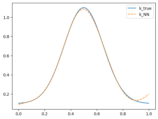
ktrue = k(x)
print("l2 relative error for k: " + str(pinnx.metrics.l2_relative_error(khat, ktrue)))
plt.figure()
plt.plot(x, ktrue, "-", label="k_true")
plt.plot(x, khat, "--", label="k_NN")
plt.legend()
plt.show()
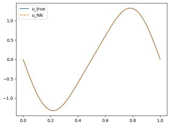
utrue = res.sol(x)[0]
print("l2 relative error for u: " + str(pinnx.metrics.l2_relative_error(uhat, utrue)))
plt.figure()
plt.plot(x, utrue, "-", label="u_true")
plt.plot(x, uhat, "--", label="u_NN")
plt.legend()
plt.show()
l2 relative error for k: 0.030291751
l2 relative error for u: 0.00095011527